Adventures in Causal Inference
I have recently read The Book of Why (TBoW) by Judea Pearl and Dana McKenzie. It is an introduction to causal inference, which estimates the impact of changes in conditions (treatments, external interventions, etc.) on outcomes using sample data. In 10 chapters, the book covers key concepts of causality and discusses the differences with mainstream statistics, with which J. Pearl’s own experience and frustrations become apparent at times.
There could have been fewer autobiographical passages but TBoW is more than a squabble between scientists as it includes multiple use cases across domains like public health or education policy. It seems that J. Pearl has been obsessed with building useful tools for practitioners by re-inventing the way we learn from data.
While reading one of the last chapters on mediation analysis, I thought of several past analytical problems where the methods described would have helped me. This blog post builds on this chapter to answer common questions an HR department may have. In what follows, I will introduce the use case, then identify direct and mediated effects, and measure these effects to estimate the impact of potential interventions.
Promotion cycles at BigBankCorp
Chapter 9 in TBoW gives an historical account of the U.C. Berkeley admission paradox, where the University’s dean wanted to know if the admission process discriminated against women. Overall admission rates were lower for females but higher or equal to males for each department.
I apply the same type of problem - known as Simpson’s paradox - using an example drawn from past experience. In my old company, Human Resources asked our team if minority employees were discriminated against during promotion rounds. This happened around the time of George Floyd’s death in the US, which prompted internal discussions about fairness for blacks and minorities in general.
Imagine that BigBankCorp, a large lending company, reviews junior staff performance on an annual basis to determine if they are ready to move to middle management positions. Human Resources want to know if the promotion process is unfair towards minority employees, which in the UK are often identified as Black Asian and Middle Eastern (BAME).
A. Identifying discrimination
BigBankCorp has almost 29,000 employees and 35% of them belong to the BAME category. A manager from Human Resources looked at the chances of promotion for each ethnic categories.
The promotion rate of BAME employees stands at 3.5%, which is about 35% lower than the rate of non-BAME employees. But, the chances of promotion by business unit (Consumer vs business-to-business) are so similar that we may think the difference would only reflect sampling variations (not true differences in means).
The results cause some confusion. The HR manager asks: “Should we double check the numbers?”
“Should I cut the data in a different way, for example, using more granular business departments?”
“What would we conclude if then percentages are similar between minorities and non? What if they show an inverse trend, as we thought would be the case?”
“Hold on, what’s the question, again?”
A causal diagram can help formulate the problem:
The diagram shows that an employee’s ethnic category influences their choice of business unit, which has an impact on promotion. We assume that B2B is BigBankCorp’s growth engine, which offers more opportunities for promotion. The question mark on the direct arrow indicates that E may or may not be a direct influence on the outcome O. A non-zero effect would be evidence of discrimination on a racial basis.
A few observations
- There must be a “mechanism” through which discrimination would happen, e.g. a bigoted assessor who sits on the promotion panel or an unconscious bias in all assessors
- Because we assume that the only other factors linked to ethnicity that influence promotions is B, what remains is discrimination; the actual mechanism doesn’t matter so we call discrimination the “direct effect”
- No arrows point into ethnic category because it’s assumed to be a genetic trait not influenced by the employee’s environment
- However, it helps to formulate the business question as if ethnic category could be manipulated - what happens to a non-BAME employee’s chances of promotions if they became BAME?
- One can further ask - if they became a BAME employee but their initial choice of business unit remains the same, what would their chances of promotions be?
To rephrase the last bullet: swapping E to BAME changes the distribution of B, but to identify a possible direct effect, we keep B the same and we ask if there remains any change in promotion outcomes.
The analytical solution is to compare promotion rates O between values of E while holding B constant. The second chart above shows no difference in outcomes, so under our causal model, there is no reason to believe that the bank’s review process discriminates on a racial basis.
In fact, the data sample behind the above charts was generated from a process where E only influences O via B.
model1 = pm.Model()
with model1:
ethnic_category = pm.Bernoulli("ethnic_category", 35 / 100.0)
p_consumer = if_else(
is_equal(ethnic_category, Employee.BAME),
# BAME
# p(department=consumer|ethnic_category=BAME) = 67%
67 / 100.0,
# Non BAME
33 / 100.0
)
business_unit = pm.Bernoulli("business_unit", p_consumer)
p_promotion = if_else(
is_equal(business_unit, Business.CONSUMER),
# Consumer
# p(outcome=promotion|business_unit=b2b) = 1.34%
1.34328358 / 100.0,
# b2b
# p(outcome=promotion|business_unit=b2b) = 7.27%
7.27272727 / 100.0
)
outcome = pm.Bernoulli("promotion", p_promotion)
We can check the absence of a direct connection by inspecting model1’s graph.
pymc3.model_to_graphviz(model1)
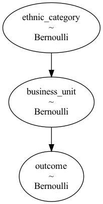
Here, every data generating process is built as a pymc3 model, a random variable that can be thought of as a template of an employee-to-outcome instance. The model defines the existence and the true magnitude of every effect, so causal analysis results can be compared to the “ground truth”.
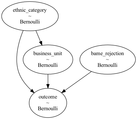
With a discriminatory process, promotion rates should be lower for BAME employees even when holding the business unit constant. To double check this, let’s emulate a direct effect using another model.
model2 = pm.Model()
with model2:
# p(E=BAME)
ethnic_category = pm.Bernoulli("ethnic_category", 35 / 100.0)
p_consumer = if_else(is_equal(ethnic_category, Employee.BAME), 60 / 100.0, 20 / 100.0)
business_unit = pm.Bernoulli("business_unit", p_consumer)
bame_rejection = pm.Bernoulli("bame_rejection", 50 / 100.0)
p_promotion = if_else(
is_equal(ethnic_category, Employee.BAME),
# BAME
if_else(
is_equal(bame_rejection, 1.0),
# Promotion is rejected
0.0,
if_else(
is_equal(business_unit, Business.CONSUMER),
# Consumer
2 / 100.0,
# b2b
8 / 100.0,
),
),
if_else(is_equal(business_unit, Business.CONSUMER), 2 / 100.0, 8 / 100.0),
)
outcome = pm.Bernoulli("promotion", p_promotion)
Discrimination happens through drop_minority_application, which randomly rejects a BAME employee’s application with a probability of 0.5. I picture a panel of case reviewers with a particularly bigoted assessor, who uses their veto power to discard one in two BAME employee application without even looking at it. The graph confirms that there is a direct effect.
pymc3.model_to_graphviz(model2)
Running the previous analysis on this model confirms the discriminatory effect. BAME candidates have a lower chance of acceptance even when holding the business unit constant.
A final note on causal model selection
- We may ask which of
model1ormodel2reflects the real selection process (if BigBankCorp was a real company), but this question sort of misses the point of a model. Models encapsulate our beliefs about the world; they are not mathematical propositions awaiting a proof. (It’s a bit more complicated because it is possible to refute a model that is at odds with the sample data observed) - Causal models should be constantly reviewed and critiqued. One could argue that other factors of promotion are missing and suggest an alternative causal diagram, which may become the new consensus
- That causal inference requires an assumption about the underlying model can be seen as a weakness, but mainstream statistics also requires assumptions for valid estimates. The need to provide a causal model is like a cost, so a question to keep in mind is “Do the benefits of causal inference compensate for its cost?”
B. Keep your “controlling urges” in check
The previous analytical approach was applied by Bikel, a statistician from U.C. Berkeley tasked with looking at the numbers to answer the question: Does the University selection process discriminate against females?
Bikel saw that admission rates by department (math, biology, etc.) were not lower for females, which he took as a decisive argument against female discrimination. But the story doesn’t stop there. TBoW tells about a conversation between Bikel and Krushke, another statistician who got interested in the case and claimed that Bikel’s analysis did not prove absence of discrimination.
Krushke built a simple numeric example to demonstrate that the same results may apply under different causal assumptions. That means that, the same data can lead to opposite conclusions depending on the causal model we hold true. I wanted to reproduce Krushke’s example, but I could not access the original document because of academic paywalls. I use TBoW’s descriptions to cook up a hopefully similar model - model3 - to prove Krushke’s point. The 3rd model is built around a type of causal effect called a collider, which the authors use to debunk a deeply anchored myth: statistical analysis should always “control for” observed variables to correctly estimate effects.
model3 is a discriminatory process that returns the same results as Query 2 from model1, where there was no discrimination. If a query returns the same results under two opposite models, then the query alone is not enough to test a hypothesis such as “BigBankCorp’s HR process is discriminatory”. Both the query and the causal model would be necessary to get the true answer. That’s an interesting lesson for organisations that pride themselves for making data-led decisions.
In model3, the source of discrimination is candidates’ citizenship (C), which takes values “local” or “expat”. The logic of discrimination is very simple: local BAME employees are always rejected, expatriate non-BAME employees are always rejected, otherwise their chances of promotion are the same. These may seem like unrealistic assumptions, but it makes the maths easier and the point would stand with smoother assumptions.
The model definition is available in the same repo. Its graph shows a direct link from E and C.
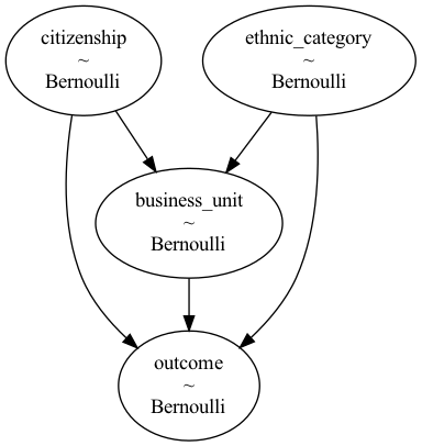
Running Query 1 and Query 2 gives the following results.
As expected, promotion rates are similar to model1. The small differences only reflect sampling variations. The expected values of Outcome are the same, i.e. we would get the same ratios with repeated sampling, which the appendix shows alongside the derivations.
Assuming that model3 is correct, how would we know if BigBankCorp discriminates against BAME employees? What query should be run against sample data?
The answer depends on the variables observed. If C is not measured, then blocking the mediation effect E->B->P is possible only with Query 1, whereas Query 2 captures both the direct and the mediated effect.
Under model3, B becomes a collider, a type of node that blocks information when not held constant, but that allows effects to flow when it’s held at a value. So, Query 2 does not answer the question because the discrimination effect E->O gets mixed up with the mediated effect E->B->O.
Colliders (click the arrow)
Colliders seem to play games with our intuitions because it's hard to accept that two independent variables can become dependent when conditioned on a third variable's value. A simple example: my cat occasionally triggers the house alarm when she plays inside and in rare instances a burglar breaking into my home would also trigger the alarm. Assume that no other factors trigger the alarm, and my cat's behaviour is independent from the burglar's. When the alarm's on, I usually think it's because of my cat so I don't panic. But, if I have left the cat at my friends' while I am on holiday, and my neighbour calls me because the alarm is on, I will think of a burglary... In other words, if I don't know the state of the alarm, then the two causal factors are independent, i.e. knowing that the cat's not at home tells me nothing about a potential thief. But, conditioned on the alarm ringing, knowing that the cat's away increases the probability of a burglary. That is, holding the collider at the value "on" allows the "cat" information to flow through and to influence my belief about "burglar".
If C is observed, then holding both C and B constant (Query 3) allows only the direct effect to propagate, so this query also tells us if there is discrimination.
Contrary to statistical folk wisdom, one should not always hold a variable constant to estimate parameters. The collider example shows that letting a collider variable freely change with its covariates can be necessary to capture the effect.
C. Measuring mediation
In the previous section we detected effects to answer questions like
Is the value zero or not?
In this section, we want to know the size of each effect to answer questions like
Does discrimination account for most of the promotion difference?
The answer, combined with BigBankCorp’s strategic goals can then inform the company’s response because direct and mediated effects command vastly different interventions.
For example, if discrimination accounts for only a small part of the promotion gap, the company may run an investigation and find the root cause to suppress it, but it may allocate the bulk of its resources to e.g. raising awareness of B2B career opportunities for BAME graduates.
Actionable insights (click the arrow)
Causal analysis aims to deliver "actionable insights", a fashionable term that most analytics projects seem to fail to deliver. This situation may sound familiar: after a team present their final results, everyone agrees that the content is "interesting", but no one is really sure what to do next. Observational data is almost always fraught with confounders, which make analysts nervous when they are asked if the data support an action, e.g. "Based on your results, do you think we should invest in/divest xyz?". Causal analysis is designed to answer interventional questions.
What follows is based on model 2. The first chart showed that the total effect of ethnic group on promotion rates is -4.9%, which we want to decompose into direct and indirect effects. The answer will appear by reframing the problem as What-If (or How many-If) scenarios. For the direct effect, we could ask
How many BAME people would have been promoted if the same proportion worked in B2B as for non-BAME employees?
Note that in this scenario, BAME promotion rates would be higher because a higher proportion will be in B2B, which has a higher promotion rate. The answer to the above question works by keeping the observed BAME promotion percentage and weighing it by the non-BAME promotion percentage, which neutralises the difference in BAME employees’ choice of business unit, i.e. it removes the indirect effect:
$p(O_p\vert E_{bame}, B_b) \times p(B_b \vert E_{non})$ for each business unit $b$.
$\sum_b p(O_p \vert E_{bame}, B_b)*p(B_b \vert E_{non}) \times 8000$ BAME individuals would have been promoted if not for the discriminatory nature of BigBankCorp’s performance process.
Then, compare this number with a baseline scenario where BAME employees get treated exactly like non-BAME employees, resulting in $p(Op \vert E_{non}) \times 8000$ promotions. The difference is the direct effect, expressed as a frequency (not as a number of individuals):
$\text{de} = \sum_b p(Op \vert Eb, BUb)*p(B_b \vert Enon) - p(Op \vert E_non)$
In the literature, the direct effect is called “natural” to refer to the baseline weights of the mediating variable, and it’s calculated by natural_direct_effect below. For BigBankCorp, the value is -3.9%, i.e. ethnic category reduces performance by c. 3.9 percentage points, or equivalently, about 3.9 percent of BAME candidates don’t get promoted solely because of discrimination. That’s about 80% of the total effect, so BigBankCorp has every reason to make the fight against discrimination their top priority.
class MediationMeasurementBinary:
def __init__(self, data):
self.data = data
# p(Op|E)
self.p1 = probability1(data)
# p(Op|E,B)
self.p2 = probability2(data)
# p(Bcons|E)
self.p5 = probability5(data)
def total_effect(self):
""" TE = p(O_p|E_bame) - p(Op|Enon)
"""
return (
self.p1["BAME"] - self.p1["NON_BAME"]
)
def natural_direct_effect(self):
""" NDE = \sum_b p(Op|Ebame, BUb)*p(BUb|Enon) - p(Op|Enon)
"""
return (
self.p2["BAME","B2B"] * (1-self.p5["NON_BAME"])
+ self.p2["BAME","CONSUMER"] * self.p5["NON_BAME"]
- self.p1["NON_BAME"]
)
We may conclude that the indirect effect is the difference between the total and the direct effect, c.1%, and we are done. NIE does is not always equal to TE-NDE, though, so let’s compute NIE from first principles then discuss why effects don’t always add up.
The solution to indirect effect works by asking
How many non-BAME employees would have been promoted if they had chosen their BUs with the same frequency as BAME employees?
Forcing a similar distribution for the mediator disables the direct effect because non-BAMEs do not suffer from any discrimination, so that would introduce only the bias owed to the choice of business unit.
The question can be translated into another data query by keeping the observed non-BAME promotion rate, $p(Op \vert E_{non}, B_b)$, and by timing it by $p(B_b \vert E_{bame}, B_b)$.
The natural indirect effect is also expressed as the difference between this simulated probability and the baseline probability $p(B_b \vert E_{non})$:
$\text{nie}=\sum_b p(Op \vert Enon, BUb)*(p(BUb \vert Ebame) - p(BUb \vert Enon))$
which estimates the number of non-BAME promotes in the hypothetical scenario that only the frequency of business units would differ. The method natural_indirect_effect computes this quantity, estimated at 2.5% for BigBankCorp.
class MediationMeasurementBinary:
# ...
def natural_indirect_effect(self):
""" NIE = \sum_b p(Op|Enon, BUb)*p(BUb|Ebame) - p(Op|Enon)
"""
return (
self.p2["NON_BAME", "B2B"]*(1-self.p5["BAME"])
+ self.p2["NON_BAME", "CONSUMER"]*self.p5["BAME"]
- self.p1["NON_BAME"]
)
That means that the choice of business unit by itself explains 2.5% of promotions, which is not miles away from the 3.9% direct effect but smaller. From an intervention perspective, this result confirms that BigBankCorp should focus on fighting discrimination, whether top management prioritise ethics or numbers published the annual sustainability report.
Non additive effects
Direct and indirect effects don’t add up if the direct effect varies with the mediator. For BigBankCorp, this means that the intensity of discrimination varies by business unit. The previous chart reveals it, as the gap between the pale brown consumer bars is smaller than the gap between the dusky purple B2B bars.
The difference between B2B and Consumer is more obvious when seen as a table
| BAME | Non-BAME | CDE | |
|---|---|---|---|
| B2B | 3.5 | 8.1 | -4.6 |
| Consumer | 0.9 | 1.8 | -0.9 |
The Controlled Direct Effect (CDE) is the difference between promotion rates at the business unit level between BAME and non-BAME, which corresponds to the question
For each business unit, what would the chances of promotion for BAME employees have been if they were treated like non-BAMEs?
which can be rephrased as
For each business unit, what would the chances of promotions for BAME employees have been if not for their ethnic category?
To emphasize discrimination. The question is similar to the NDE’s, only at the business unit level. The corresponding query works by holding the business unit (i.e. the mediator) constant and comparing promotion rates. About 4.6% of BAME individuals in B2B were not promoted due to discrimination, and this is over 5 times higher than in Consumer, so the direct effect clearly interact with mediation and effects are not additive.
As a side note, that result can be surprising because in model2, discrimination is built in through a flat 50% rejection rule via drop_minority_application. This design suggests that discrimination does not vary by business unit, although after more careful inspection this is only true in the log-probability space, as the CDE then becomes
$\log {0.5 \times p(Op \vert E_{non}, B_{b})} - \log p(Op \vert E_{non}, B_{b}) = log {0.5}$
for each business unit b. So, the results from the sample are consistent with the data generative process.
For information about effect interactions, my main source was Pearl (2014), as on this topic, TBoW’s high-level descriptions left me with more questions than answers.
Implications for interventions
If HR at BigBankCorp remove discrimination before next year’s round of promotions, there will only remain the indirect effect. So, if the Head of HR believes that a successful intervention will close the promotion gap between ethnic categories, the analyst should revise their expectations - ending discrimination will reduce the gap, but there will remain an expected difference of c.2.5% difference owing to employees’ business unit choices. With no direct effect, all that remain are indirect effects, which by themselves amount to an expected 2.5% of BAME employees. The literature refers to this measurement as the sufficient cause for indirect effects, i.e. excluding any direct mechanism.
Similarly, 3.9% is the sufficient cause for direct effect (excluding any mediation mechanism). The difference between total effects and sufficient causes is called necessary. For example, the necessary mediation effect here is 4.9-3.9=1.0, which corresponds to what discrimination on its own can’t explain, i.e. the part of the direct effect that relies on mediation to exist.
Final comments
In TBoW, the authors refer to the “Causal Revolution” as the effort to build a unified theory for causal analysis and its proliferation over the last few decades to disciplines like econometrics, epidemiology or psychology.
Part of me thinks that the word “revolution” is too strong to describe what seems to be a range of useful analytical tools. These tools improve our understanding of existing problems/concepts like mediation analysis or confounders but a revolution suggests a more radical transformation.
I could be wrong and causal inference may open up completely new possibilities. For example, machines may finally start learning - as a human, not a sophisticated mimicry - when they distinguish between correlation and causation.
Counterfactuals, a language developed to express causal notations that probability has always struggled with, is particularly exciting. It is beyond the scope of this blog post, which focusses more on intuitions than formalism, but I will briefly show how counterfactuals apply to the net direct effects computed before.
\[\text{nde} = \sum_b{p(O=p \vert E=bame, B=b)}*p(B=b \vert E=non) - p(O=p \vert E=non)\]This expression would read better if we could combine the terms inside the summation into a joint probability and invoke the total law of probability to have one nice probability. The notation does not allow it because employees refer both to BAME and non-BAME individuals, but counterfactuals make this possible by writing
\[\sum_b{p(O_{E=bame, b} \vert B_{E=non}=b}) \times p(B_{E=non}=b)=\sum_b{p(O_{E=bame}=p, B_{E=non}=b)}\]with subscripts referring to the ethnic group, so this is the probability of the joint events that an employee chooses their business unit with the same distribution as non-BAME but get promoted as BAME.
The sum spans all values of b, so it becomes $p(O_{E=bame, B_{E=non}}=p)$, and if promotion is 1 and rejection is 0, the probability for promotion is also the expectation of $O$, $E(O_{bame,B_{non}})$, using a simplified counterfactual symbols. Applying the same logic to the second term in the nde formula,
\[\text{nde}=E(O_{bame,B_{non}} - O_{non,B_{non}})\]Quite a rich idea in a compact formula.
References
- D. Mackenzie and J. Pearl (2018). The Book of Why.
- J. Pearl (2014). Interpretation and Identification of Causal Mediation.
Appendix 1
I use pymc3 to craft and sample from imaginary Data Generatin Processes (DGPs). The true parameters of this DGP can then be compared with causal inference estimates.
Simulated data - or fake/dummy/synthetic data - can be generated using scipy or numpy’s random variables, which is fine for simple DGPs like a multivariate gaussian, but beyond this I find the code unreadable. Probability graphs are easier to read because they define the process for one observation, and the sampling method takes care of the rest.
pymc3 might sound overkill for this, because I don’t need any bayesian inference functionality just to create DGPs, but the library interface is simple and it comes with useful tools like diagram visualisation.
A bayesian probabilistic graph is a set of conditional probability distributions (CPD) for each node. (starting nodes like Citizenship are just prior probabilities, i.e. not conditioned on any variables). To get a DGP, I need to define each node’s probability distribution, conditioned on the depending nodes. For example, Business Unit ($p(B_b \vert C_c, E_b)$) is a Bernoulli rv defined for all 4 cases corresponding to the values that (C, E) can jointly take.
Defining a DGP in this way means that constraints can be enforced by expressing them as CPDs defined in the graph. See the next appendix for details.
Appendix 2
To prove that there exists a discriminatory model, called model3, that returns the same query results a the non-discriminatory model model1, the following must be true
- Requirement 1: in
model1andmodel3promotion promotion rates by business unit must be the same for each ethnic group - Requirement 2: promotion rates for BAME employees must be lower than for non
- Requirement 3: the expected value of the probabilty of promotions must be the same for both models
Notation
$O_p$: Outcome=promoted
$E_b$: Ethnic group=BAME ($E_{non}$ for non-BAMEs)
$C_{ex}$: Citizenship=expatriate ($C_l$ for locals)
$B_{cons}$: Business unit=Consumer ($B_{b2b}$ for business-to-business)
The constraints are
Requirement 1
For every b in {Consumer, b2b}
\(p(O_p \vert E_b, B_b) = p(O_p \vert E_{non}, B_b)\)
For Consumer, this expression implies
I skip the details, but it’s essentially integrating out and using the fact that we set $p(O_p \vert B, E_{non}, C_{ex})=0$ and $p(O_p \vert B, E_b, C_l)=0$.
Then, $p(C_{ex} \vert E_b, B_b)$ can be expanded into an expression that takes CPDs that we set: $\frac{p(B_b \vert C_{ex},E_b) \times p(C_{ex})}{\sum_c(p(B_b \vert E_b, C_c) \times p(P(C_c))}$. So, I get a value for $p(O_p \vert D, E_{non}, C_l)$ that I can set in the graph.
Requirement 2
The overall chances of promotion are lower for BAME employees:
$p(O_p \vert E_b) < p(O_p \vert E_{non})$
That one’s interesting. The expanded form is
\[\sum_b p(O_p \vert E_b, C_{ex}, B_b)\times p(C_{ex})\times p(B_b \vert C_{ex}, E_b) < \sum_b p(O_p \vert E_{non}, C_l, B_b)\times p(C_l)\times p(B_b \vert C_l, E_{non})\]The middle terms, $p(C)$, can be ignored because we assume that there are fewer expatriates, so $p(C_{ex})<p(C_l)$. The remaining two probablilities are that of getting promoted conditioned on ethnicity and business unit, times that of the chosen business unit given E.
The first probability is already fixed to meet requirement 1, so it’s out of my control. I tried some substitutions, but I failed to get an expression that would garantee that the requirement is met, and the best I could do is to guess a value and do the calculation to check if the requirement is met. We can come up with a good guess, though - if b2b has a higher promotion rate than Consumer, then setting a higher probability of Consumer for BAME employees will mechanically reduce their promotion rates compared to non-BAMEs.
That’s essentially Simpson’s paradox in full force, because as shown on model3’s chart, promotion rates conditioned on E and B are higher for BAME employees than non-BAMEs, and yet, requirement 2 is also true.
Requirement 3
$p(O \vert E)$ and $p(O \vert E, B)$ must be similar in model1 and model3.
This is guaranteed by inputing model3’s CDP into model1, using $p(B \vert E)$ and $p(O \vert E,B)$, which can be easily derived. For example
$p(B_{b2b} \vert E_{bame})=\sum_{c}{p(B_{b2b} \vert E_{bame}, C_c) \times p(C_c)}$.
Empirical checks
It’s possible to verify that requirements are met by way of sampling. That approach was not available in 1970s, when all statistical work had be done by hand, so we should be grateful and use our inexpensive computers.
For the example of Requirement 1, let’s sample say, 50 datasets, and compute $p(O \vert E_{bame}, B_b)-p(O \vert E_{non-bame}, B_b)$, for each business unit. probability4 does it for one sample dataset.
def probability4(data):
""" p(promotion | E_bame, B_b) - p(promotion | E_non, B_b)
return
(pd.Series) The difference in promotion rates for b2b and consumer
"""
return (
probability2(data)
.rename("promotion")
.reset_index()
.pivot(
index="business_unit",
columns="ethnic_category",
values="promotion"
)
.sort_index()
.assign(difference=lambda df: df["BAME"]-df["non-BAME"])
.loc[:, "difference"]
)
Repeating this 50 times and looking at the results confirms that the chances of promotion by business unit are the same for each ethnic category. The sample distributions are clearly centered around 0. If still in doubt, just draw more samples!