Improving Shapley values with Causal Knowledge
The SHAP explanation method has been widely used because of useful guarantees, availability across frameworks and a sense of accessibility/flexibility. The most sought-after property is local accuracy, which guarantees that the sum of Shapley values match the difference between a prediction and a baseline value. There are fast implementations with good documentations across many frameworks, for example shapr, used in this blog. Finally, SHAP does not seem to require assumptions about the underlying data process and some implementations like KernelSHAP apply to any ML model.
In practice though, it can return misleading results, which I will illustrate in the first part with two examples. The second part looks at Shapley values as a combination of scenarios and identifies unhappy scenarios that we may want to exclude. Scenario exclusion should agree with any causal knowledge of the underlying data. The last part introduces Asymmetric Shapley values to add causal assumptions to improve Shapley values.
This blog post assumes some familiarity with SHAP as covered in introductions like the Interpretable ML online book.
A. (Unexpected) Results
Two examples will illustrate when SHAP may return unexpected results
- A variable is not used, also called a non-interventional variable
- A variable is determined by a parent variable, a case of variable mediation
To anchor the examples, I will use a classic loan approval use case. A financial institution is about to launch an automated loan approval product but they ask us to audit the model first to make sure that it complies with regulation. They want to understand what variables are used to predict a loan outcome. We are told that the only predictor used by the model is the applicant’s income, but we also have data about the applicant’s race and favourite TV show.
To assess Shapley values, we build our own data generative process, which reflects how the bank has run its loan application business for many years. A sample of past applications are used to train an ML model, which we want to audit with Shapley values.
Writing our own synthetic datasets creates expectations to assess Shapley results against. At a minimum, explanations should capture the racial bias built into the process, but other aspects like the range of values will also serve as expectations.
Non-interventional
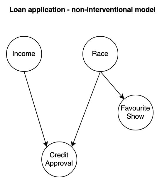
Diagram of the Data Generative Process (DGP) for the non-interventional example: a loan outcome is determined by the applicant’s Income and their Race. Their favourite TV show is caused by Race but isn’t an input into the outcome. If this causal model seems absurdly simplistic or weird, it probably is but the implications we’ll draw are applicable to more realistic scenarios.
g_non_interventional <- function(N){
	income <- 1 + 3*rnorm(N)
	race <- 1 + 5*rnorm(N)
	favourite_show <- race + rnorm(N)/2
	y <- 0.5*income + 0.5*race + rnorm(N)
	return(cbind(income, race, favourite_show, y))
}
g_non_interventional implements the generative logic with only numeric variables for simplicity. If you prefer thinking about categorical variables, for example “1: Loan application approved ; 0: Loan application not approved”, you can assume variables like raceand y to be described in the log-odds space, then we could apply an inverse logit transform to describe them as probabilities.
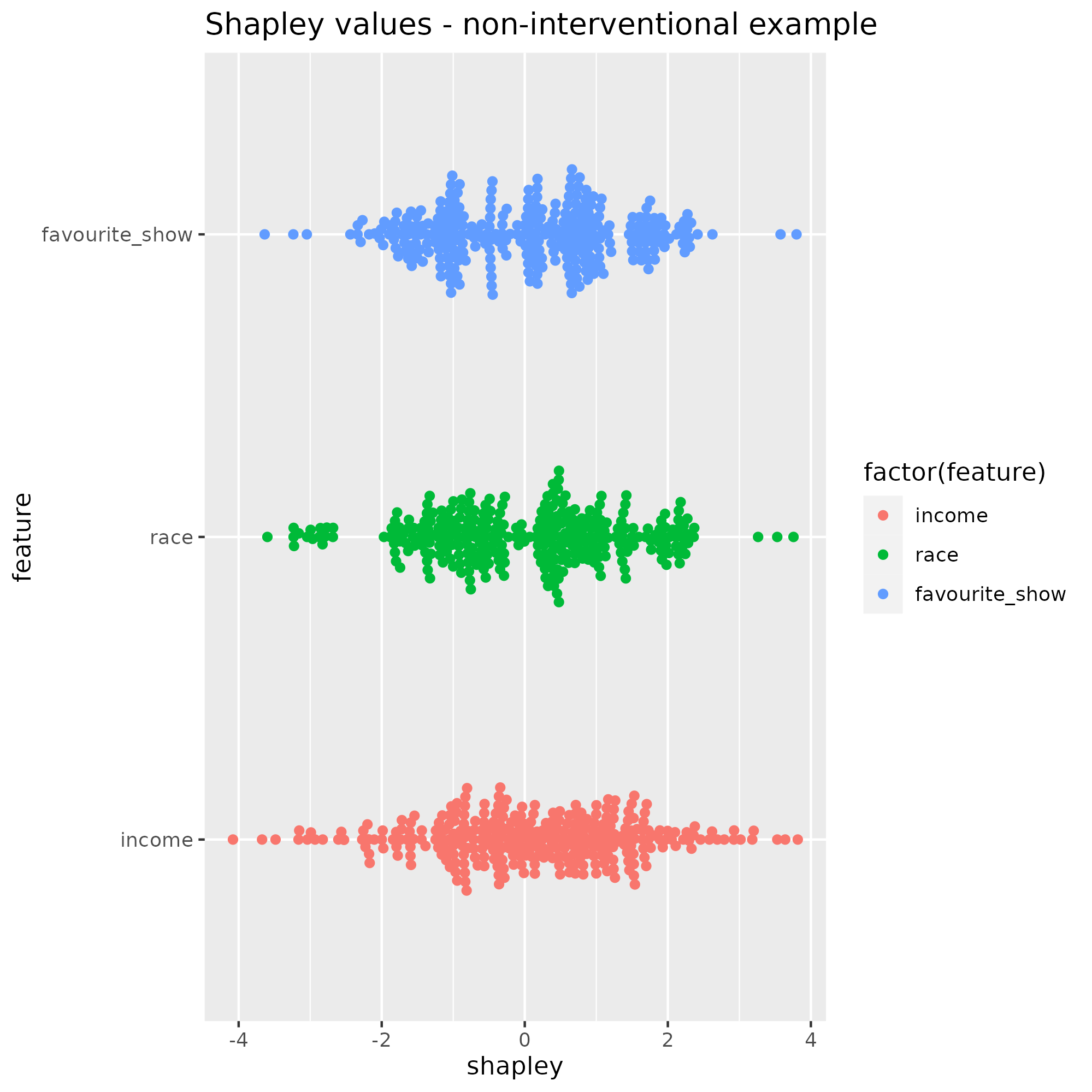
Next, we train an ML model and generate 300 obervations from this DGP to apply KernelSHAP and plot the distribution of shapley values for all 3 variables income, race and favourite_show.
Shapley value distributions span the same range for all three variables, meaning that favourite_show gets attributions often as large as the other two variables although it’s not an input into the loan outcome. If we didn’t know it, would we conclude that Netflix preferences partially determine an applicant’s access to credit? Thinking beyond this exammple, Shapley values of non-interventional variables can be different than zero, which can lead analysts to the wrong conclusions.
Mediation / Indirect effect
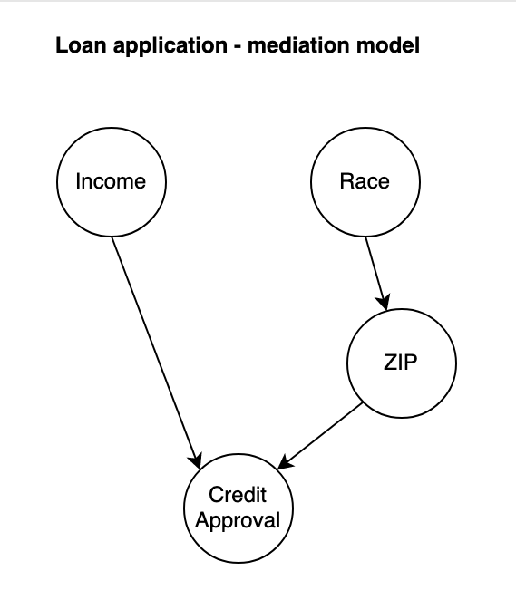
The next example keeps Income and Race and introduces Zip Code as a mediation variable. Race determines an applicant’s zip code area but it has no direct effect on the loan approval outcome. Income and Zip code are the inputs into the loan approval outcome.
g_indirect_effect <- function(N){
    income <- 1 + 3*rnorm(N)
    race <- 1 + 5*rnorm(N)
    zip <- race + rnorm(N)/5
    y <- 0.5*income - 0.5*zip + rnorm(N)
    return(cbind(income, race, zip, y))
}
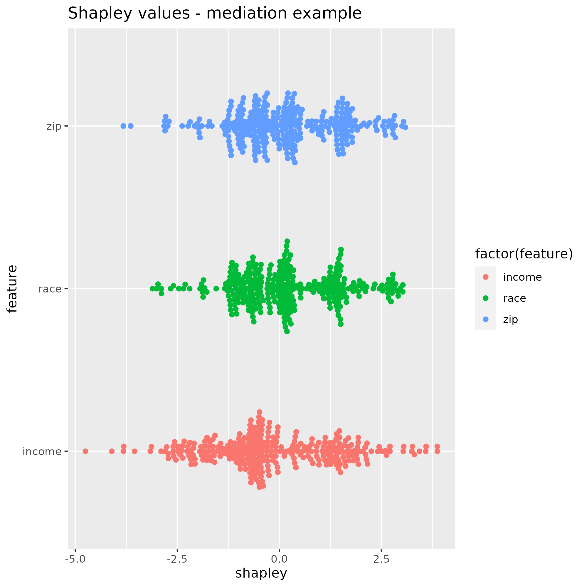
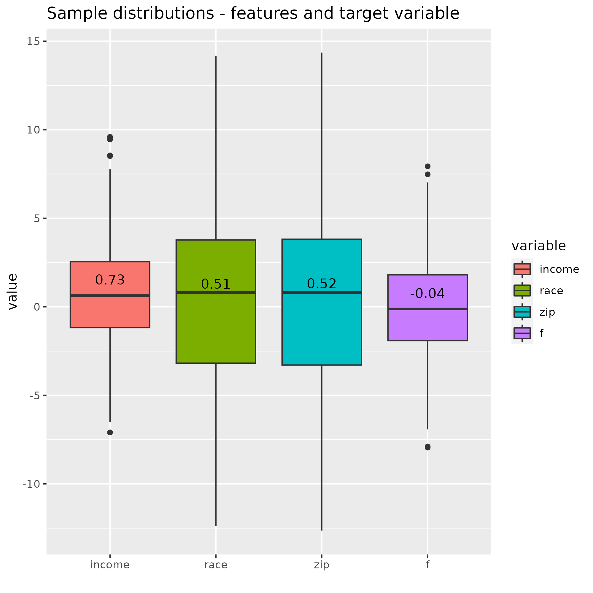
g_indirect_effect implements the causal model. Higher income and lower race values increase the chances to get the loan approved. The distribution of race Shapley values should be more spread out than that of income because its random error is 1.6x larger. Also, the explanation attributed to zip code should not be zero because, though this variable is mostly determined by race, it has a small random component, i.e. a small effect on the loan outcome that can’t be attributed to race.
The same ML model as before is trained and kernelSHAP is run on 300 observations. Shapley value distributions show, again, that all three variables have the same range. This means that the zip code “explains” the loan outcome as much as race does, although it is predominantly determined by race. Here we would expect race to have more explanatory power than zip code overall, so it seems that SHAP dilutes the true effect of race with the zip code.
Shapley values underestimate the true effect of race, which hides the actual discrimination. An auditor may wrongly conclude that a model is compliant because sensitive attributes appear to have less explanatory power than they really have, due to the effect being spread over child variables. We need to correct Shapley values for such situations.
B. Shapley as an overage of scenarios
Shapley and scenarios
SHAP explains a prediction by taking each feature and estimating what the predicted value from model f would have been without this feature. The comparison involves many scenarios corresponding to coalitions of features. Every scenario is like a single experiment that attempts to answer the question “How much does the feature contribute to the prediction?”. A feature’s Shapley value combines all the answers into a single value.
In other words, the Shapley value averages scenarios to provide a contrastive explanation Δ(i). Δ explains why we shouldn’t drop feature i (assuming Δ is not zero, else it can be dropped). The explanation could be worded like “You can’t drop feature i because it changes the prediction by Δ(i) from the baseline”. The baseline can be any reference value and is often chosen to be the expectation $\mathbb{E}(f(\text{X}))$.
The chain of contrastive statements “explain out” the prediction with reference to the baseline value, a property sometimes called local accuracy because SHAP describes exactly how, starting from the baseline expectation, each feature contributes to the final prediction.
The problem is that for every feature, some of the scenarios that Shapley averages over may not be consistent with our knowledge of the data generating process. We would therefore like to ignore inconsistent scenarios. Section C gives an example of how we can be selective about these scenarios to improve Shapley values.
To recap with some notations
- A coalition, denoted S, is a group of features used to predict an instance. In-coalition features are part of the model whereas out-of-coalition features are excluded
- The Outcome function or payoff function is a model’s prediction under a coalition, written $v_{f,x}$ where f is the predictive model and x are in-coalition features
- A scenario is an outcome under a particular coalition, i.e. Δ_v(i, S) where i is the target feature for a prediction. For example, Δ_v(zip, {income, race}) assesses the change in f when zip code is added to a coalition of income and race
- $\phi_i$ is the Shapley value of feature i, the average over all possible scenarios:
\(\phi_i = \frac{1}{\text{M}}\sum_{S\subseteq M\setminus \{i\}}{M-1 \choose \vert S \vert}^{-1}(v(SU\{i\})-v(S))
\tag{1}\)
- $v(SU{i})-v(S)$ reports a single experiment’s result, which is run for all possible coalitions S and averaged such that smaller and very large coalitions carry more weight, because ${M-1 \choose \vert S \vert}^{-1}$ is a U-shape function of the number of elements $\vert S \vert$.
- Local consistency is the guarantee that the sum of Shapley weights is equal to the difference between a prediction and a baseline value like $\mathbb{E}(f(\text{X}))$.
Zip code example
The scenarios are built from all coalitions that exclude zip, of which there 2^(N-1) so 4
\[\{\varnothing\} , \{\text{income}\}, \{\text{income, race}\}, \{\text{race}\},\]The scenario under the empty set evaluates the impact of adding the zip code when there is no features. The no-feature outcome is the prediction of the expected value for every feature, $f(\mathbb{E(X)})$, estimated as the average prediction over the training set; the outcome when only zip code is present can be estimated with a sample of the remaining features conditioned on the known value for zip. We will come back to the estimation of out-of-coalitions features.
Another interesting scenario is built on the 3rd combination that includes income and race. Looking at the effect of the zip code when income and race are known can tell us if zip code has any explanatory power at all because all other features are included. $\Delta_v$ captures any remaining effect of zip after everything else has been accounted for. \(Δ_v(\text{zip}, \{\text{income, race}\})=v_f(\{\text{income, race, zip}\}) - v_f(\{\text{income, race}\})\)
Let’s take an example by an applicant called Erick, to illustrate this scenario. Erick has an average income, low race values and a high prediction of acceptance.
| value | |
|---|---|
| Income | 0.9571218 |
| Race | -4.655322 |
| Zip code | -4.646968 |
f |
2.58386 |
Compare these values with all test observations to add some perspective.
We want to calculate $Δ_v(\text{zip}, {\text{income, race}})$.
$v_f,x({\text{income, race, zip}})$=$f(x)$=2.584 because it’s the prediction when all features are in the coalition. What would be the outcome without zip, $v_f,x({\text{income, race}})$? If it is the same as $f(x)$ then the difference Δ_v is zero and zip would make no contribution. For Erick, $v_f,x({\text{income, race}})$=2.687, which is close to the predicted outcome. A statistical test does not allow to conclude that the two values are different, which reinforces the view adding the zip code has no effect on the prediction.
Another interesting scenario is S={race}, the coalition with only race. Here again, the data supports the hypothesis that $\Delta_v$ is zero, so the zip code has no incremental effect when race is already factored in. That’s two out of four scenarios that don’t attribute any effect to zip.
In Erick’s case, the Shapley value for zip is 1.104 though, so clearly not zero. In the chart below, each bar shows the Shapley values for one of the three features and the baseline, “None”. The number next to the feature name corresponds to its actual value in the dataset. Most of the explanation is attributed to the combined effect of zip code and race. All values add up to the applicant’s predicted value of 2.584 owing to Local accuracy.
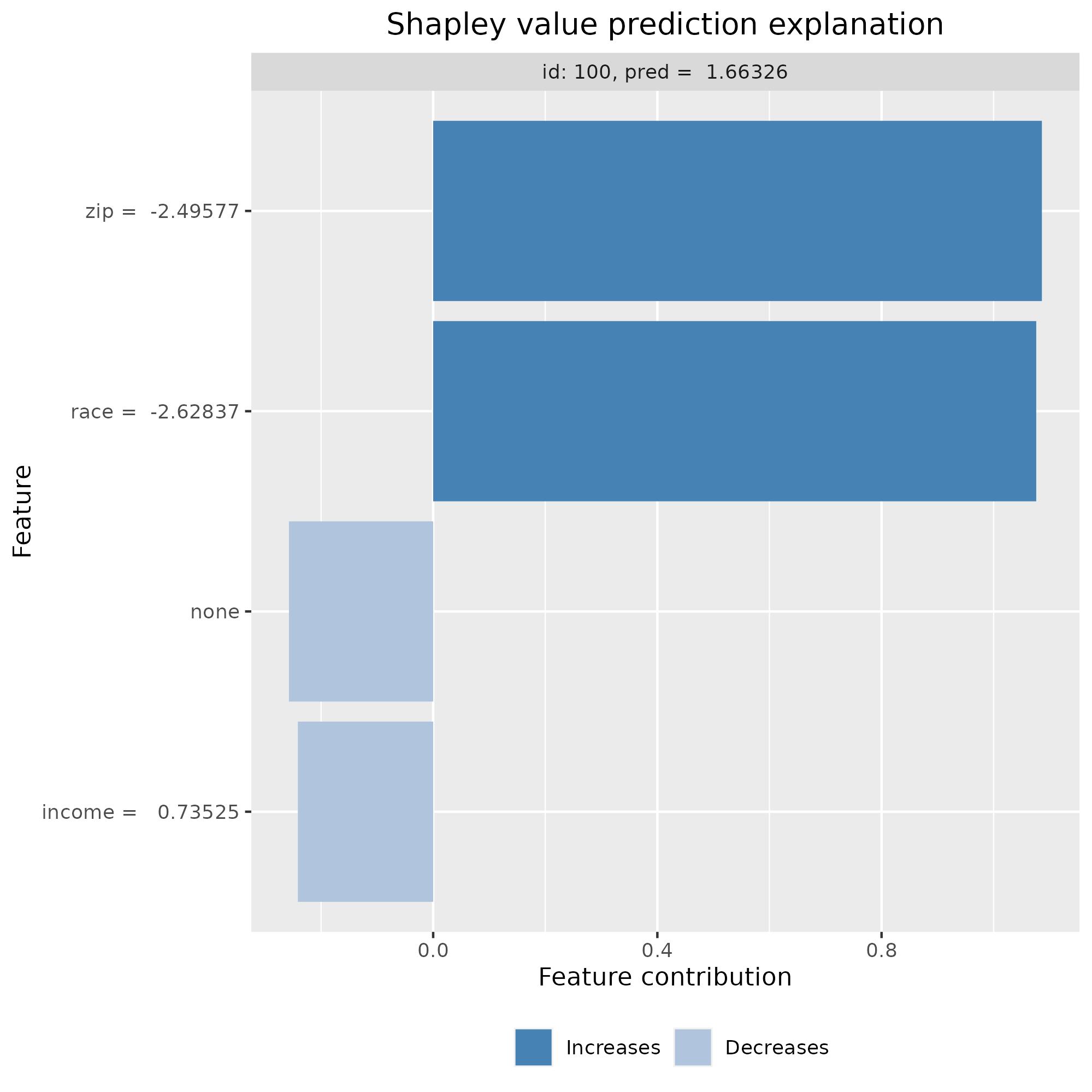
From the Shapley formula, $\phi_{zip}$ must be different than zero because of the scenarios based on ${\varnothing}$ and ${\text{income}}$. Each of these scenarios captures the effect of zip when race is missing, which passes its effect onto the zip code, which acts as a proxy for race.
If we know that race is a causal ancestor of the zip code, then we want $\phi_{zip}$ to only measure the additional effect of zip when race is known, not the effect of an imaginary scenario where zip code acts like race. Asymmetric Shapley value allows to precisely capture this effect, while keeping Local accuracy. It’s covered in section C, just after clarifying a few things about out-of-coalition features.
Estimating Shapley outcome functions $v_{f,x}$
To get $v_{f,x}$ we can retrain the same model keeping in-coalition features, e.g. $v_{f,x}({\text{race}})$ by dropping income and zip code. But training 2^M models where M is the number of features wouldn’t be efficient in many cases, so we average the model predictions on a sample of likely values for out-of-coalition features. For example, if only race is known, the “likely” values of income and zip are determined by $p({\text{income, zip}} \vert \text{race})$.
Shapley has no opinion on how the outcome function is calculated or what the feature distribution is, so we make the best decision possible. Here the features are known to be generated from a normal distribution so I use shapr’s multivariate Gaussian but this package has other options - parametric and otherwise - available. Worth noting that some packages only provide empirical estimates by independently sampling each feature, which makes samples prone to unrealistic hallucinations. For example, if features include smoking behaviour and age, sampling independently may
include 5-year old chain smokers, which the model is not trained to adequately respond to - what would an adequate prediction even mean?
To recap, $v_{f,x}(\text{race})$ is approximated with $E_{X_{\text{income, zip}} \vert X_{\text{race}}}f(x_{\text{race}}, X_{\text{income, zip}})$, the expected prediction with respect to the probability of income and zip (out-of-coalition features) conditioned on the known value of race. $x$ is the known value and $X$ are the conditional distribution values. The other outcome function $v_{f,x}(\text{race, zip})$ is also estimated and the sample distributions strongly overlap.
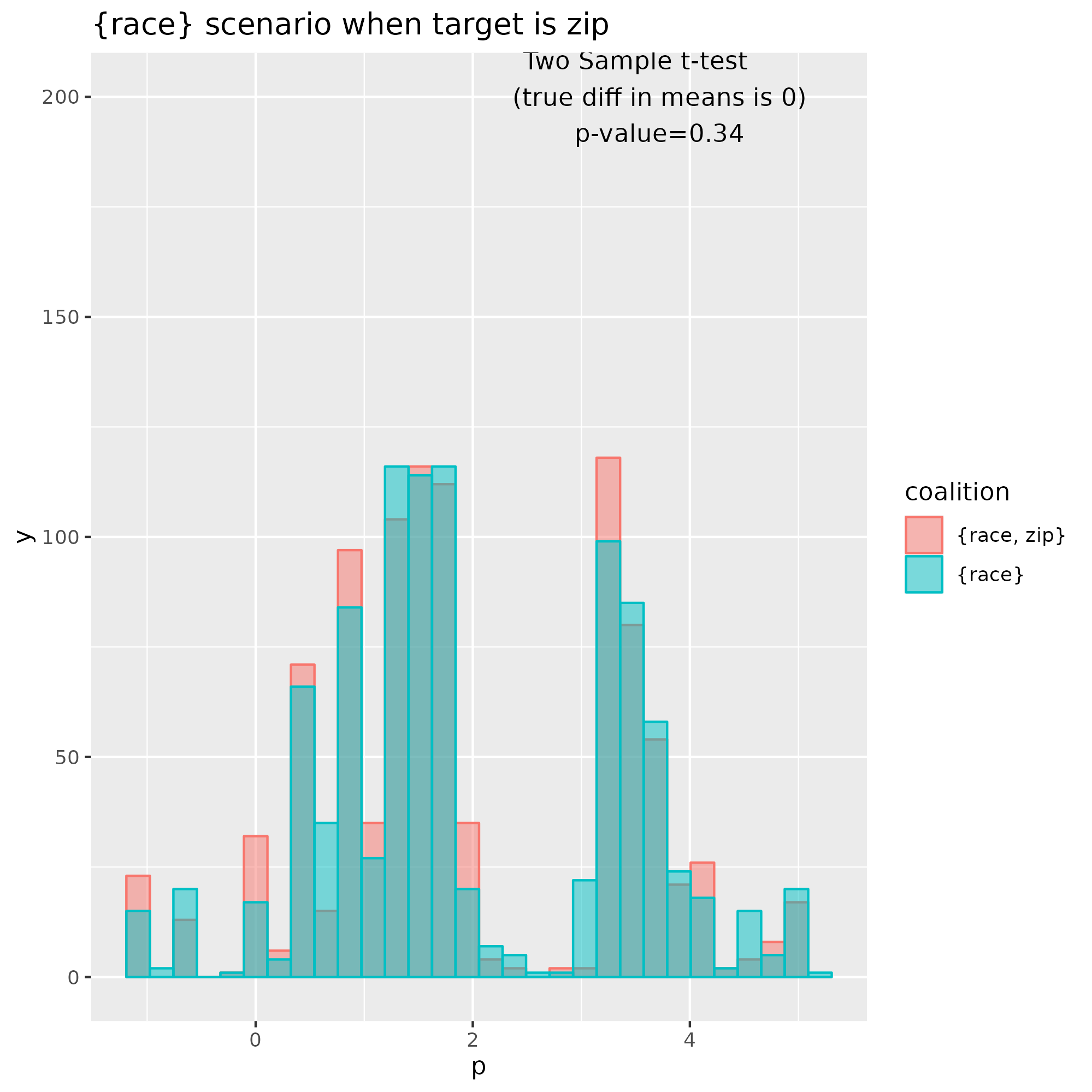
A t-test for the difference in mean gives a p-value of c.0.34, supporting the view that \(\Delta_v(\text{zip}, \{\text{race}\})\) = 0 i.e. that zip code has not incremental effect on the prediction when only race is known.
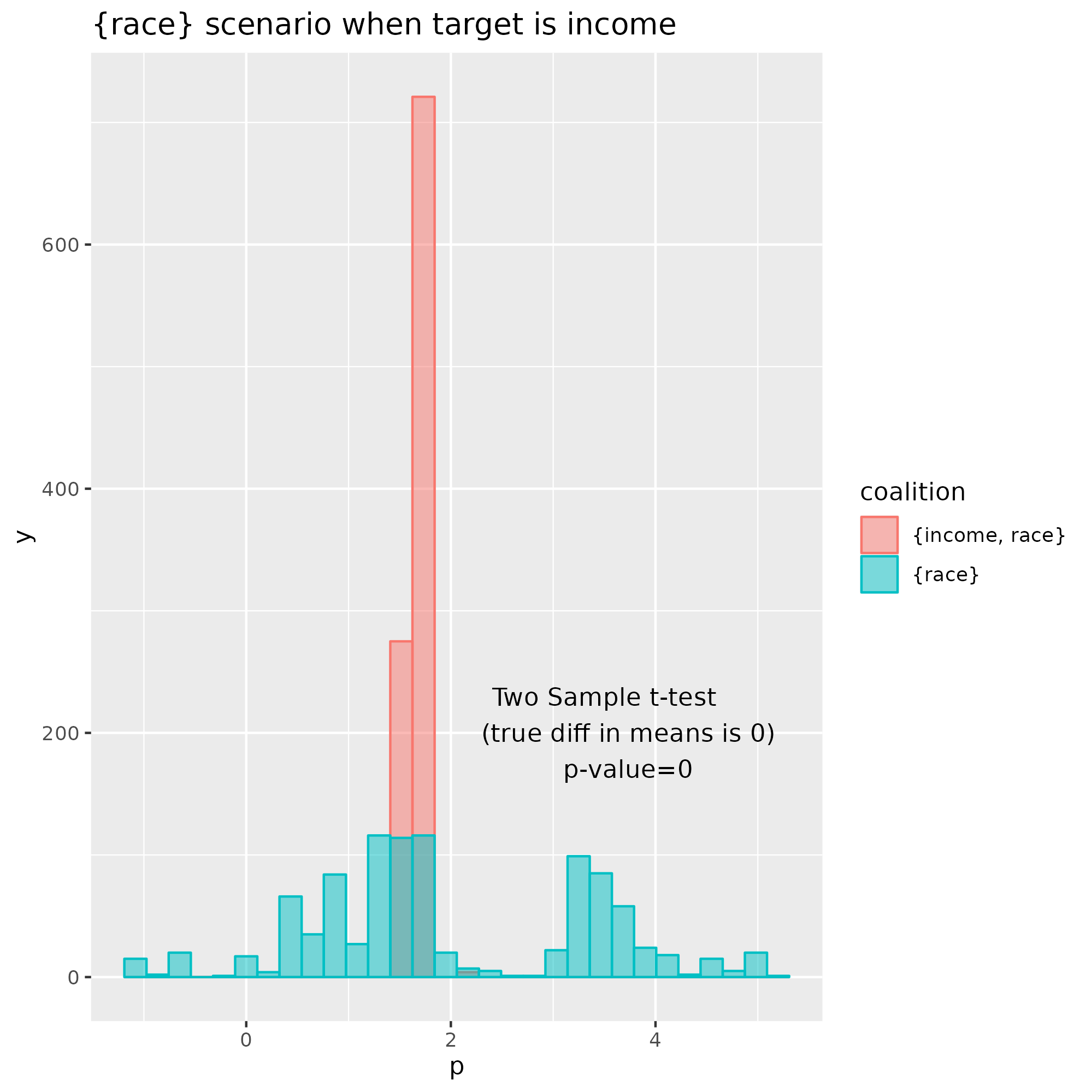
To contrast this example with another scenario that captures a real effect, take for example \(\Delta_v(\text{income}, \{\text{race}\})\). The sample distributions are different and the p-value of the t-test supports the opposite conclusion as before.
C. Asymmetric Shapley values
(Expected) Results
Asymmetric SHAP incorporates causal information into the calculation of Shapley values. For example, if we add the constraint that race comes before zip code is known, then $\phi_{race}$ will capture the total effect of race on the loan outcome, either directly or through the zip code, and $\phi_{zip}$ captures any remaining effect when race is already present. Any causal relationship can be added to adjust Shapley values - we don’t need to provide a full causal graph.
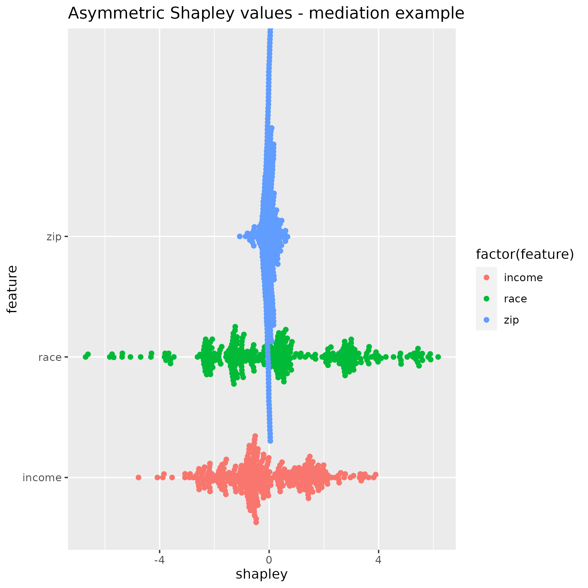
After adjusting Shapley values with the causal pattern “Race -> Zip -> Loan outcome”, the range of Shapley values for zip code shrinks and the range of Race increases, in line with the data generation process. The range of income values is smaller than that of race, which reflects its lower error variance.
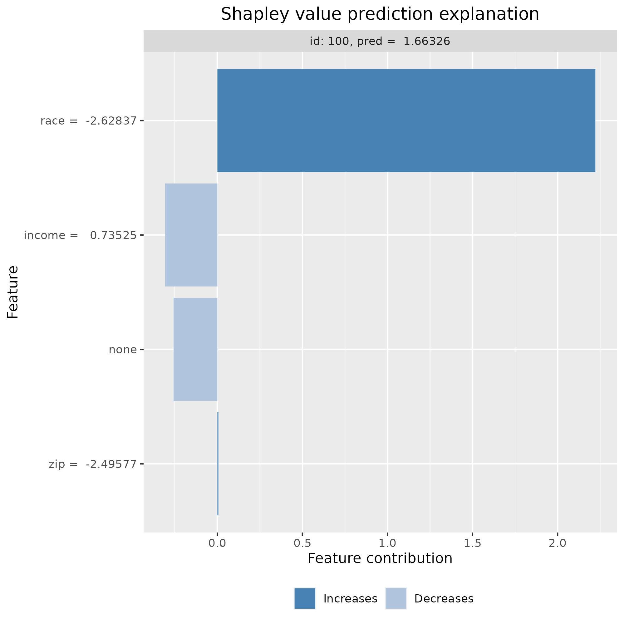
For Erick’s application, most of the explanation goes to race rather than income, which reflects Erick’s race score being in the 10% lowest value vs his income that is around the test sample average. Zip code is close to zero, so its value under symmetric Shapley was transferred over to race. The sum of all weights remains equal to the loan outcome prediction because local accuracy still applies under asymmetric Shapley values.
How it works
I will try and provide some intuitions on the implementation of asymmetric Shapley used for this blog. For more information, in particular about the mathematical foundations behind it, I would refer to the original article.
We want to ask more specific questions than “What’s the effect of [target feature] on the predicted value?”. For example, “What is the incremental effect of adding zip code to race on the predicted value?”. That question agrees with our causal model of the data, as we know that race is an ancestor of zip code in the graph/lineage. Some scenarios don’t help answer a refined question, for example the case based on the empty coalition, where \(\Delta_v(\text{zip}, \{\varnothing\})\) does not include the effect of race.
Asymmetric Shapley gives us control over the scenarios by adjusting their weights depending on causal relationships. To get a look into its mechanics, we need to think about scenarios from feature ordering rather than coalitions, i.e. from (ordered) permutations rather than (unordered) combinations. If $t_{\text{zip}}$ builds a coalition using all variables that come before zip, e.g.
$t_{\text{zip}}$(income|race|zip, excl) = {income, race}
$t_{\text{zip}}$(income|race|zip, incl) = {income, race, zip}
$t_{\text{zip}}$(zip|race|income, excl) = {$\varnothing$}
$t_{\text{zip}}$(zip|race|income, incl) = {zip},
then a Shapley value is a sum of all orderings with equal weights.
For example, $\phi_{\text{zip}}$ = $\frac{1}{6}$ (v(t(zip|race|income, incl)) - v(t(zip|race|income, excl)) ) +
$\frac{1}{6}$ (v($t_{\text{zip}}$(zip|income|race, incl)) - v($t_{\text{zip}}$(zip|income|race, excl)) ) +
$\frac{1}{6}$ (v($t_{\text{zip}}$(income|race|zip, incl)) - v($t_{\text{zip}}$(income|race|zip, excl)) ) +
$\frac{1}{6}$ (v($t_{\text{zip}}$(income|zip|race, incl)) - v($t_{\text{zip}}$(income|zip|race, excl)) ) +
$\frac{1}{6}$ (v($t_{\text{zip}}$(race|zip|income, incl)) - v($t_{\text{zip}}$(race|zip|income, excl)) ) +
$\frac{1}{6}$ (v($t_{\text{zip}}$(race|income|zip, incl)) - v($t_{\text{zip}}$(race|income|zip, excl)) )
The sum is over six elements corresponding to all 3! permutations, each assigned the same weight $\frac{1}{3!}$. We can then map every item to a scenario, e.g. the first two orderings correspond to the empty coalition. Side note - staring enough at the permutation and the combination formulas helped me understand where the weights from the formula come from.
One flavour of asymmetric Shapley, called proximal, allows to assign weights of 1 to orderings that agree with our (partial) causal model, such that
$\phi_{\text{zip_asymmetric}}$ =
$\frac{1}{3}$ (v($t_{\text{zip}}$(income|race|zip, incl)) - v($t_{\text{zip}}$(income|race|zip, excl)) ) +
$\frac{1}{3}$ (v($t_{\text{zip}}$(race|income|zip, incl)) - v($t_{\text{zip}}$(race|income|zip, excl)) )
$\frac{1}{3}$ (v($t_{\text{zip}}$(race|zip|income, incl)) - v($t_{\text{zip}}$(race|zip|income, excl)) ) +
The 3 elements that the Shapley value sums over correspond to scenarios based on the coalitions {income, race} and {race}, which we have shown to be close or equal to zero.Therefore, $\phi_{\text{zip_asymmetric}}$ is small or equal to zero.
Open questions
Asymmetric Shapley values, or alternative approaches to improve vanilla Shapley like Causal Shapley, have a lot of potential to become part of the mainstream Responsible AI toolkit. The original article shows creative and useful applications for time series or feature selection. But a few questions would need to be answered before using it for real use cases.
First, it does not have the user community that standard Shapley provides, e.g. R’shapr in R or python’s shap, where people answer each other’s questions and contributors keep the projects active. In fact, I wrote a script based on the equations from the article because I could not get the authors’ library to work for my example.
Then, it’s not clear how it would scale beyond a few hundred observations. The implementation just mentioned uses Monte Carlo sampling, which sounds good but may trade off accuracy for efficiency.
Last, without a process to capture and validate causal knowledge, there is a risk of implementing wrong causal assumptions, which could be as bad as not using any. One organisational challenge I have seen is the functional isolation of teams delivering Shapley solutions - often software engineers or data scientists, which have no or low interactions with subject matter experts who have a mental model of causal relationships.
Conclusion
Standard Shapley value implementations can behave unexpectedly with correlated features, which recent causal-based methods like asymmetric Shapley can resolve. A Shapley value averages many scenarios that test the impact of a feature on the predicted value. When we look more closely into the list of scenarios considered, some do not ask relevant questions. I think of asymmetric Shapley as a way to take control of the scenarios to ask the right question.
References
- C. Frye, C. Rowat and I. Feige (2020). Asymmetric Shapley values: incorporating causal knowledge into model-agnostic explainability.
- E. Kumar, S. Venkatasubramanian, C. Scheidegger and S. Friedler (2020). Problems with Shapley-value-based explanations as feature importance measures.
- D. Janzing, L. Minorics and P. Blöbaum (2019). Feature relevance quantification in explainable AI: A causal problem.
- L. Merrick1 and A. Taly (2020). The Explanation Game: Explaining Machine Learning Models Using Shapley Values.