Introduction to Expectation-Maximization and Latent Variable Models - part 1
This post introduces a framework to estimate latent variable models using a real-life scenario example with a simple univariate probability distribution. The second part builds on the following intuitions and equations to explore other latent models and show what they have in common.
Motivations
EM overview
A model with latent variables assumes that sample data are generated by one of many components. Typically, components are random variables of the same probability distribution, e.g. Poisson or Gaussian, each with different parameters. Components are also generated by a random variable that can be discrete, as with Gaussian mixture model (GMM), or continuous, as with variational autoencoders (VAE).
Expectation-Maximization (EM) is a framework to estimate the parameters of such models. It is an alternative to direct optimisation using Maximum likelihood estimation (MLE), which is straightforward for single distribution models. MLE is an intuitive, widely used method that asserts that the best estimates are those that explain the evidence — the sample observations — with the highest probability.
Why latent variable models?
They give superpowers to the single distribution models we are familiar with by accounting for the heterogeneity of the underlying populations, even if no attribute indicates group membership.
Single distributions try to fit many diverse profiles into a one-size-fits-all model. It is like trying to fit one shoe size to different feet. In contrast, mixture models allow us to try and fit different sizes so long as the shoe model remains the same.
In my experience applying these models at work, for example in the context of behavioural analysis or privacy-preserving ML, I could get high accuracy with a reasonably simple architecture. That allowed me to get the job done and be able to communicate the results to various audience types.
With latent variables it is possible to train generative models, i.e. estimate the full distribution of a data generating process, with high accuracy. In my personal experience, the range of applications of generative models is broader than that of traditional ML models.
Note on model inference
Typically, ML models are concerned with the relationship between a target and a set of predictors. They essentially perform a correlation on steroids, which is great if you need an accurate forecasting tool. For any other application, generative models may be more suitable, for example in synthetic data generation or data clustering.
In what follows the “model” will refer to a random process represented as a joint probability distribution of two random variables (RV). The generative process for an observation starts with a sample from the latent RV, which gives $t$, followed by a sample from the corresponding mixture RV, which gives $x$. The goal is to estimate the parameters of the joint probability distribution of $x$ and $t$.
A univariate example
Let’s consider the following scenario — Kate manages a restaurant that offers seating and home delivery. She thinks that the kitchen staff may be under-resourced to address sudden spikes in home deliveries between 7-8 pm. She wishes to compute the probability distribution of 7-8 pm delivery orders to inform her resourcing decisions.
Deliveries are managed by a 3rd party aggregator app that provides the number of orders placed over 10 min intervals. The chart below describes the number of orders for Mon-Thu over 3 weeks i.e. 12 days shown on the x-axis.
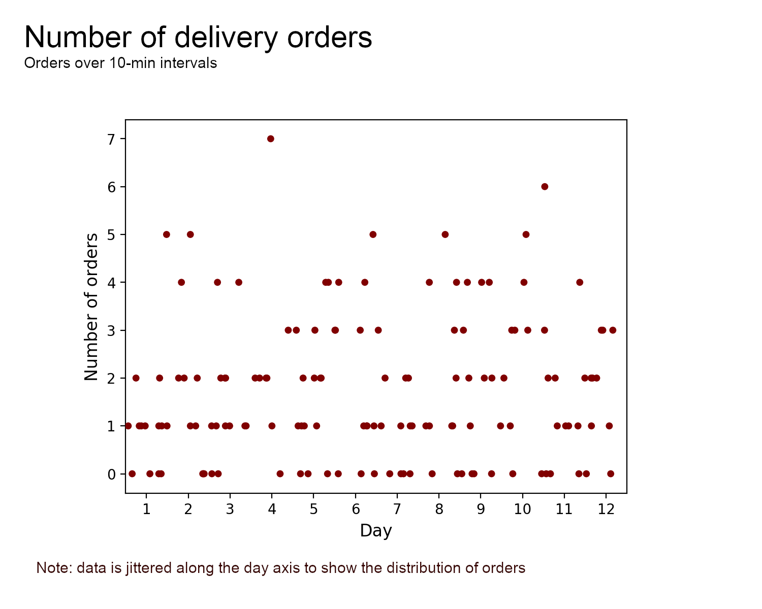
We can assume that orders are independent events occurring at a constant rate between 7-8 pm. Kate assumes Fridays behave differently so doesn’t consider orders on this day for her model. At first glance, she may use a Poisson process to model this data however she suspects that the two delivery companies available, Uber Eats and Deliveroo, may have different order rates.
Unfortunately, the aggregator logs do not break down the data by delivery company, which can thus be thought of as latent variables. This is an example where going from a single to a mixture of distribution models can help capture the underlying process more accurately.
Expectation-Maximization (EM) can be used here to estimate models with latent variables. To understand the strengths of EM, it is useful to start by assuming that components are observed rather than latent to estimate the parameters $\theta$ with MLE and then compare with the EM solution.
Observed Variables
If we observe $t_i$, the delivery company, then the likelihood function for the number of orders is
\[\prod_{i=1}^N\prod_{t=1}^2 P(x_{i}, t_{i}=c) =\] \[\prod_{i=1}^N\prod_{t=1}^2 P(t_{i}=c)P(x_{i} | t_{i}=c)\]Where
- N is the number of observations
- ${x_i}$ is the number of orders placed over a 10-min interval, and
- ${t_i}$ is the delivery company that manages the order i.e. Uber Eats (${t_i}=1$) or Deliveroo (${t_i}=2$)
Using the indicator $[t_i=c]$ that is 1 if component 1 generated the observation, and 0 otherwise, and using ${\pi_c}$ to denote $P(t_{i}=c)$ the likelihood becomes
\[\prod_{i=1}^N\prod_{c=1}^2 \{\pi_c\frac{\lambda_c^{x_i}}{x_i!}e^{-\lambda_c}\}^{[t_i=c]}\]To be clear our goal is to find $\hat\theta$, the estimate of $\theta$ which maximises the likelihood function. In this scenario there are 4 parameters, two priors and two Poisson parameters so $\theta = (\pi1, \pi2, \lambda1, \lambda2)$.
The next step is to apply a logarithm to simplify the expression. The log-likelihood is
\[\begin{equation} \sum_{i=1}^N\sum_{c=1}^2 {[t_i=c]}\{\log\pi_c+x_i\log\lambda_c-\lambda_c-\log(x_i!)\} = \tag{1.1} \end{equation}\] \[\sum_{c=1}^2{n_c}\log\pi_c+\sum_c^2\sum_i^N\{x_{ic}\log\lambda_c-\lambda_c-\log(x_{ic}!)\}\]Where ${n_c}$ is the number of observations assigned to component c and $x_{ic}$ is short for $[t_i=c]*x_i$
Taking the derivative wrt $\lambda_c$ gives a simple solution for the Poisson parameter (the rate of orders)
\[\sum_i^N\frac{x_{ic}}{\lambda_c} - {n_c} = 0\] \[\begin{equation} \lambda_c = \frac{\sum_i^Nx_{ic}}{n_c} \tag{1.2} \end{equation}\]Which means that the parameter for a component is its average value, which is the same result as the single Poisson distribution.
For the component probability $\pi_c$, add the constraint that probabilities must sum to 1 through a Lagrangian denoted with parameter $\delta$. The log-likelihood is then
\[\sum_{c=1}^2{n_c}\log\pi_c + \sum_{c=1}^2\sum_i^N\{x_{ic}\log\lambda_c-\lambda_c-\log(x_{ic}!)\} + \delta(\sum_{c=1}^2\pi_c - 1)\]The derivative wrt to $\pi_c$ is
\[\frac{n_c}{\pi_c} + \delta = 0\]Multiply by $\pi_c$ on each side, sum over $c$, and remember that the sum of probabilities is 1 to get $\delta = -N$. Then
\[\pi_c = \frac{n_c}{N} \tag{1.3}\]That means that the prior probability $P({t_i=c})$ is the proportion of observations from component $c$ over all observations $N$.
Latent Variables with MLE
If we can’t observe component $t_i$ then things get complicated. At first, likelihood estimation seems possible because we can write the likelihood function, $\prod_{i=1}^N P(x_i|\theta)$, by integrating out the hidden variables.
If we can write the objective function, can we optimise it though? Let’s see. The likelihood is
\[\prod_i^N\sum_c^2P({x_i},{t_i}) =\] \[\prod_i^N\sum_c^2P(t_{i}=c)P(x_{i} | t_{i}=c)\]And the log-likelihood is
\[\begin{equation} \log P(X|\theta) = \sum_i^N\log\sum_c^2P(t_{i}=c)P(x_{i} | t_{i}=c) \tag{1.4} \end{equation}\]As explained in PRML:
The presence of the sum prevents the logarithm from acting directly on the joint distribution, resulting in complicated expressions for the maximum likelihood solution.
One can ignore this warning and try and solve the above heads-on but it will not be a simple exercise.
Next, we will show that using EM is a better alternative because it is simple and it works well with latent variables and distributions of the exponential family.
Latent Variables with EM
Imagine that Kate’s best friend works at the food delivery aggregator app and can provide some information about delivery companies. He’s got a model to estimate the probability of the component given the observation $P(t=c \vert {x_i})$.
In plain English, he has a black box that takes a number of orders in a 10-min interval and outputs the probability that the orders are managed by Uber Eats or Deliveroo. We can use this posterior distribution to get a formula for the log-likelihood that’s almost like the complete-data formula.
\[\begin{equation} \sum_{i=1}^N\sum_{c=1}^2 P(t_i=c|x_i)\log P(x_i, t_i=c) = \tag{1.5} \end{equation}\] \[\sum_{i=1}^N\sum_{c=1}^2 P(t_i=c|x_i)\{\log\pi_c+x_i\log\lambda_c-\lambda_c-\log(x_i!)\}\]Note how similar the last expression is to the expression in 1.1. The indicator variable is replaced by the posterior, i.e. our best guess for the true component that generated ${x_i}$.
I think of equation 1.5 as a “quasi complete-data” likelihood function, a state of knowledge that is halfway through the complete-data (omniscient) and the incomplete-data (ignorant) states. In the literature, it is sometimes referred to as the “expectation of the complete-data” likelihood and denoted $\mathcal{Q}$.
The log-likelihood function can be solved for $\theta$ because the $\log$ “acts directly on the joint distribution”. Let’s unpack this.
Solving for $\lambda_c$
\[\sum_i^N(\frac{P(t_i|x_i)}{\lambda_c}x_i - 1) = 0\] \[\lambda_c = \frac{\sum_i^NP(t_i|x_i)x_i}{\sum_i^NP(t_i|x_i)} \tag{1.6}\]The solution is close to the solution in 1.2. It is the average weighted by the membership assignments. We don’t know which component $x_i$ comes from so we use the best approximation available, $P(t_i \vert x_i)$.
The latent component solution for the prior probability includes the same steps seen before. Using a Lagrangian and setting the derivative wrt. $\pi_c$ gives
\[\sum_{i=1}^N \frac{P(t_i=c|x_i)}{\pi_c}+ \delta = 0\]And the solution is
\[\pi_c = \frac{\sum_i^NP(t_i|x_i)}{N} \tag{1.7}\]The prior probability for a component is the proportion of observations from that component, using the posterior probability as an approximation for membership assignment.
We have estimated $\hat\theta$, which corresponds to the “M” step of Expectation-Maximization. Kate can use the mixture of Poisson estimates to support her business decisions.
For example, if her restaurant is open for take-away from 7 pm she can estimate the probability of having at least 5 orders in the first 20 minutes or, using the relationship between Poisson and exponential distributions, she can evaluate the probability that the first requests will occur after 7.10 pm.
Furthermore, if Kate thought that her friend’s black box programme can be further refined she could use $\hat\theta$ to “update” the posterior probabilities using Bayes’ rule
\[P(t_i=c|x_i)=\frac{P(x_i|t_i=c,\theta)P(t_i=c)}{\sum_j^2P(x_i|t_i=j,\theta)P(t_i=j)} \tag{1.8}\]All the ingredients on the RHS of this equation are available. The chart below illustrates the relationship between mixture parameters and the posterior distribution. Assume that $(\pi_1, \pi_2, \lambda_1, \lambda_2) = (0.54, 0.46, 0.957, 2.626)$
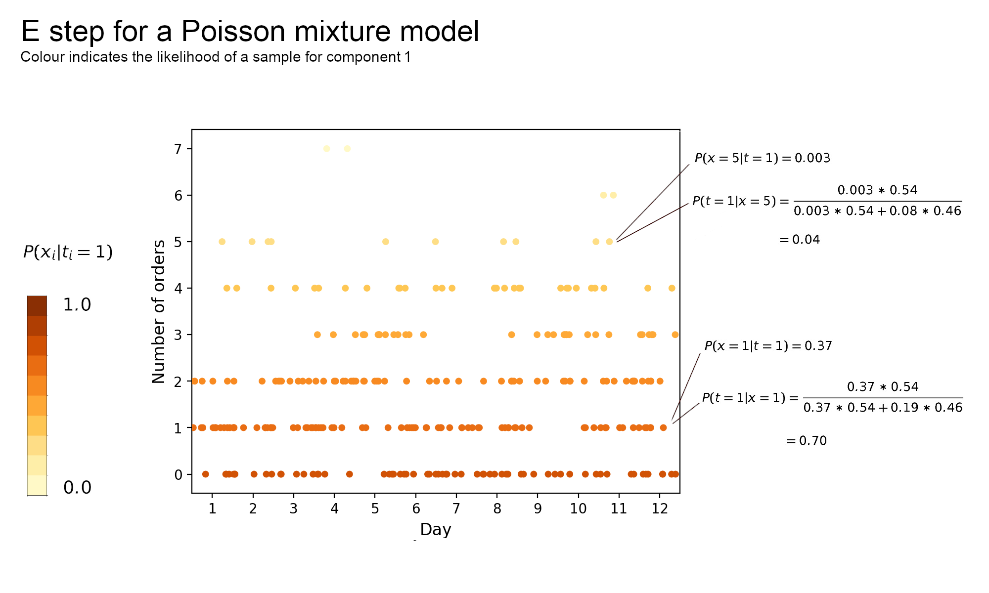
Looking at component 1 the posterior probability for $x=1$ is high at 0.7 whereas 5 orders are less likely to come from this component with a probability of 0.04. With prior probabilities roughly the same, posterior probabilities are close to the likelihood hence the results above make sense. The likelihood of component 1 is higher than component 2 around $x=1$ as its parameter, which is also its expected value, is close to 1.
Expectation-Maximization
The imaginary example above suggests why Expectation-Maximization is useful. It’s an optimization programme used to estimate parameters for probability distributions with latent variables when your best friend can’t provide reasonably good estimates of the posterior $P(t=c \vert {x_i})$.
EM addresses the same problem as MLE but takes a different, iterative approach to it. As shown before MLE quickly stumbles upon a complex expression whereas in the M step Kate worked around it using the “quasi complete-data” likelihood i.e. the expectation of the complete-data likelihood. At this stage three questions are left unanswered:
- Where does the “quasi complete-data” function come from?
- How do I get a good posterior probability distribution?
- What guarantees of convergence to a maximum does EM provide?
The short answers are
- It's a lower bound for the likelihood function
- Start with random values then iterate through the E and M steps
- There's no guarantee of global maximum, however EM will lead to points with zero valued gradients
The 3rd answer implies that EM can get stuck in local minima or saddle points, which is unsatisfying, so in practice EM goes through several iterations to only keep the best estimate.
The detailed answers require to first define a lower bound for the log-likelihood probability. The maths gets a little dry but the code implementation will hopefully make it more palatable.
The lower bound
The log-likelihood function can be written as the sum of two functions, $L$ and $KL$ for any value $\theta$ and any probability distribution $q$
\[\log P(X|\theta) = L(\theta, q(t_i=c)) + KL(q(t_i=c)\parallel p(t_i=c|x_i,\theta)) \tag{2.1}\]With
\[L(\theta, q) = \sum_i^N\sum_c^Nq(t_i=c)\log p(x_i, t_i=c|\theta) - \sum_i^N\sum_c^Nq(t_i=c)\log q(t_i=c) \tag{2.2}\]And
\[KL(q(t_i=c)\parallel p(t_i=c|x_i,\theta)) = -\sum_i^N\sum_c^Kq(t_i=c)\log\frac{p(t_i=c|x_i,\theta)}{q(t_i=c)}\]$L$ is a lower bound for the log-likelihood, a function that is at most equal to $\log P$ for any $\theta$ and $q$. That is because $KL$, the Kullback Leibler measure of divergence, is greater than or equal to zero. Just like the smallest possible distance between your home and your office is zero, the smallest possible divergence between $q$ and the posterior probability distribution is zero in which case $q(t_i=c) = p(t_i=c \vert x_i,\theta)$.
$q$ is a probability distribution function over the latent variable $t_i$, in this case a probability mass function i.e. something that takes discrete values $(t_1, t_2, …, t_K)$ and maps them to [0, 1] with the constraint that $\sum_c^Kt_c=1$. A particular realisation of $q$ is the posterior $p(t_i=c \vert x_i)$ but the expression above is true for any distribution function, e.g. $(0, 0, … 1)$ or $(\frac{1}{K}, \frac{1}{K}, … \frac{1}{K})$.
The point of this decomposition is that the lower bound has nicer mathematical properties than the log-likelihood and $KL$ is easy to reason with. So instead of an ugly objective function we have two attractive expressions.
The appeal of the lower bound is apparent when optimising wrt $\theta$ as she can be written as $\sum_i^N\sum_c^Nq(t_i=c)\log p(x_i, t_i=c \vert \theta) + C$ which is the expression in 1.4.
$KL$ is handy because, for a fixed value of $\theta$, she is equal to zero when $q$ is equal to the posterior probability. The EM game is about alternating between $L$ and $KL$ until we reach the apex of the log-likelihood. The details and code example will be served after the proof of the decomposition.
Proof of the decomposition
The proof starts from the $KL$ divergence and breaks it down to get equation 2.1. First, separate out the ratio inside the $\log$ and apply Bayes’ theorem to the posterior $p(t_i=c \vert x_i,\theta)$
\[\begin{equation} \begin{aligned} KL(q(t_i=c)\parallel p(t_i=c|x_i,\theta)) & = -\sum_i^N\sum_c^Kq(t_i=c)\log\frac{p(t_i=c|x_i,\theta)}{q(t_i=c)} \\ & = \sum_i^N\sum_c^Kq(t_i=c)\log q(t_i=c) - \sum_i^N\sum_c^Kq(t_i=c)\log \frac{p(t_i=c, x_i|\theta)}{p(x_i|\theta)} \end{aligned} \end{equation}\]Further split out the fraction inside the $\log$ on the RHS expression, rearrange the resulting terms and use the fact that $p(x_i \vert \theta)$ does not depend on c and $\sum_c^K q(t_i=c)=1$ as $q$ is a distribution. The $KL$ divergence is equal to
\[-(\sum_i^N\sum_c^Kq(t_i=c)\log p(t_i=c, x_i|\theta)+\sum_i^N\sum_c^K q(t_i=c)\log q(t_i=c))+\sum_i^N \log p(x_i|\theta)\]So $KL$ is the sum of minus the lower bound $L$ (LHS) plus the marginalised log-likelihood $\log P(X|\theta)$ (RHS). Rearranging gives equation 2.1 above, which breaks down the log-likelihood into the lower bound and the $KL$ divergence.
EM with code implementation
In equation 2.2., the posterior distribution includes the mixture parameters that we seek to estimate - see 1.8. EM resolves this chicken-and-egg problem by addressing the posterior probability and the mixture parameters separately.
It starts with random initialisation of either membership assignment or the parameters, then alternates between updating the membership assignment given the parameters and updating the parameters given the membership assignments.
After each round the log-likelihood increases, and this goes on until there is no longer any significant increase.
Let’s look at each step in detail.
Initialisation
Start with a random guess of $\theta_0$ to kick off the iteration process. The code implementation uses different heuristics for the parameters. The prior probability $\pi_c$ is set at a fixed value of $\frac{1}{C}$ while $\lambda_c$ is assigned a random draw from a Poisson RV with a rate parameter equal to the sample average.
def random_init_params(mixture_init_params):
    '''
        Initialise mixture distribution parameters.

        \pi_c is initialised as 1/C i.e. components
        have the same prior probability to be drawn.
    '''
    def general_random_init_params(X, C):
        D = X.shape[1]
        pi = np.ones(C) / C
        mixture_params = mixture_init_params(X, C, D)
        return (pi, ) + mixture_params
    return general_random_init_params

def mixture_init_params_poisson(X, C, D):
    '''
        Initialise Poisson mixture param by drawing
        samples from a Poisson RV with rate equals to the
        sample mean.
    '''
    return (poisson(mu=np.mean(X, axis=0)).rvs(C).reshape(C, 1), )

random_init_params_poisson = random_init_params(mixture_init_params=mixture_init_params_poisson)
E step
Objective: optimise the lower bound $L$, wrt the posterior probability $q$, using the mixture parameters $\theta$ fixed at the value from the previous step.
Solution:
\[q = p(t_i=c \vert x_i, \theta) \tag{2.3}\]In equation 2.1 $\log P(X \vert \theta)$ does not vary with $q$ so $L$ is maximised when the KL divergence is minimised i.e. $q = p(t_i=c \vert x_i)$. If $L$ is a set of red marbles, $KL$ blue marbles and $\log P(X \vert \theta)$ is a jar, the only way to fill up the jar with red marbles is to remove all the blues.
With a Poisson mixture, equation 2.3 is equivalent to equation 1.8. The function e_step below returns q / np.sum(q, axis=-1, keepdims=True) which is the solution in 1.8 because q, assigned one line above, is the joint probability of $t$ and $x$.
This snippet also demonstrates that EM works flexibly across different probability distributions that can just be plugged into the general E step function. In the next part of this blog article, poisson_likelihood will be replaced with a Gaussian likelihood function.
def e_step(likelihood: Callable) -> Callable:
    """
    Implements the E step of the EM algorithm.

    Args:
    likelihood: The mixture probability function
                e.g. Poisson, binomial or multivarite normal

    Returns:
        The posterior distribution for observations X using
        the mixture parameters estimated in the M step
    """
    def general_e_step(X, pi, distribution_params):
        N = X.shape[0]
        C = pi.shape[0]

        q = np.zeros((N, C))

        for c in range(C):
            q[:, c] = likelihood(c, distribution_params, X) * pi[c]
        return q / np.sum(q, axis=-1, keepdims=True)
    return general_e_step

def poisson_likelihood(c: int, mixture_params: Tuple[Any], X: np.array) -> np.array:
    """

    Args:
    c: Component index
    mixture_params: Distribution parameters i.e. prior proba
                    and Poisson rate
    X: Observations

    Returns the Poisson probability mass for X
    """
    lambda_param = mixture_params[1]
    return poisson(lambda_param[c]).pmf(X).flatten()

e_step_poisson = e_step(likelihood=poisson_likelihood)
M step
Objective: optimise the lower bound $L$, wrt the mixture parameters $\theta$, using the membership assignments computed in the previous step i.e. setting $q$ as $p(t_i=c \vert x_i)$.
Solution:
\[\begin{equation} \begin{aligned} \DeclareMathOperator*{\argmax}{argmax} \argmax\limits_{\theta} L(\theta \vert q) = \argmax\limits_{\theta} \sum_{i=1}^N \sum_{c=1}^Kq(t_i=c)\log p(t_i=c, x_i \vert \theta) + C \end{aligned} \end{equation} \tag{2.4}\]This is the lower bound function defined in 2.2 with the quantity that does not vary with $\theta$ denoted as a constant. 2.4 is equivalent to the expectation of the complete-data likelihood in 1.5.
The actual results depend on the mixture distribution but the presence of the $log$ next to the joint distribution makes the solution straightforward for any distributions of the exponential family.
For a Poisson mixture, the solutions to 2.4 are 1.6 and 1.7 which are implemented below.
def m_step(mixture_m_step):
    def general_m_step(X: np.array, q: np.array) -> Callable:
        """
        Computes parameters from data and posterior probabilities.

        Args:
            X: data (N, D).
            q: posterior probabilities (N, C).

        Returns:
            mixture_params, a tuple of
            - prior probabilities (C,).
            - mixture component lambda (C, D).
        """

        N, D = X.shape
        C = q.shape[1]

        # Equation 1.7
        pi = np.sum(q, axis=0) / N

        mixture_params = mixture_m_step(X, q, C, D)

        return (pi, ) + mixture_params
    return general_m_step

def mixture_m_step_poisson(X: np.array, q: np.array, C: int, D: int) -> Tuple[np.array]:
    '''
        M step for a Poisson mixture. Implements equation 1.6.

        Returns:
            The updated lambda parameter (C, D).
    '''
    lambda_poisson = q.T.dot(X) / np.sum(q.T, axis=1, keepdims=True)
    return (lambda_poisson, )

m_step_poisson = m_step(mixture_m_step_poisson)
Evaluate $\log P(X|\theta)$
Using the estimated parameters, evaluate either the log-likelihood or $L$, and stop if there is no significant increase from the previous round. The code implementation measures $L$, defined in the lower_bound function.
The convergence check happens in the train function with iteration stopping if the current change in lower bound is less than the tolerance threshold rtol.
if prev_lb and np.abs((lb - prev_lb) / prev_lb) < rtol:
    break
Convergence
Finally, what guarantees do we have that EM will converge? After each iteration $\log P(X \vert \theta)$ can only be equal or above its previous value because it is greater than or equal to the optimised lower bound (M step), which is greater than or equal to the non optimised lower bound (E step), which is equal to the previous log-likelihood.
It may help to visualise the explanation.
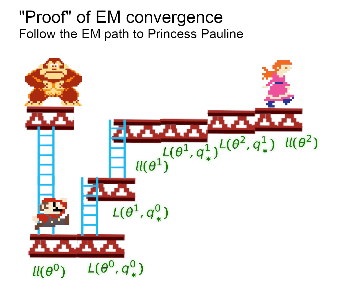
$ll$ refers to the log-likelihood and $q_*^d$ is $P(t=c \vert x_i)$ with $d$ being the iteration round. If Mario chooses the EM path, he will either go uphill or flat, but not down. In this case he will find Pauline after only 2 EM rounds.
The alternative path (MLE) goes straight up, which is tempting, but he will have to put up a fight with Kong. Mario is not after the shortest path, he just wants to find his fiancé, so he’ll choose EM.
References:
- C. Bishop. Pattern Recognition and Machine Learning (PRML).
- HSE online course. Bayesian Methods for Machine Learning.
- Code is hosted on Github, and is mostly based on Martin Krasser’s notebook.