Introduction to Expectation-Maximization and Latent Variable Models - part 2
A mixture of Gaussians
The first part introduced the EM algorithm as an alternative to direct MLE optimisation for models with latent variables. This part builds on the previous Poisson mixture example to look at other models to apply EM, e.g. Gaussian mixtures, or where elements of EM help to understand the optimisation scheme, e.g. Variational Autoencoders.
EM for GMM
The difference between a Poisson and a Gaussian mixture is that the observed data is assumed to be normally distributed, so $P(x_{i} \vert t_{i}=c)$ has two parameters, $\mu_c$ and $\sigma_c^{2}$. The log-likelihood 1.4 from part 1 is
\[\sum_i^N\log\sum_c^2P(t_{i}=c)P(x_{i} | t_{i}=c) = \sum_i^N\log\sum_c^2\pi_c\mathcal{N}(x_i|\mu_c,\Sigma_c) \tag{3.1}\]There are 6 parameters to estimate vs. 4 with Poisson distributions
\[\theta = \{\pi_1, \pi_2, \mu_1, \mu_2, \Sigma_1, \Sigma_2\}\]The EM programme described in the previous part will provide the solution to $\theta$.
Initialisation
Initialise $\theta$ using random or fixed values. For example, $\mu$ can be sampled from a normal distribution centered around the sampling average of the data set, and the $\pi$ coefficients can be set at 0.5 each.
E step
Updating equation 2.3 with a multivariate normal density function gives
\[P(t_i=c|x_i)=\frac{\mathcal{N}(x_i|\mu_c,\Sigma_c)\pi_c}{\sum_j^2\mathcal{N}(x_i|\mu_j,\Sigma_j)\pi_j} \tag{3.2}\]M step
As with the Poisson mixture, the solution for $\theta$ is not too far from the single distribution results albeit with membership assignments acting as weights.
Solving for $\mu$, equation 2.4 gives
\[\sum_i^N\sum_c^2P(t_i=c|x_i)\{\log\pi_c-\log Z-\frac{1}{2}\frac{(x_i-\mu_c)^2}{\Sigma_c}\} \tag{3.3}\]where $Z$ is a constant wrt $\mu$. Setting the derivative to 0, the solution is the sample average weighted by the posterior probability
\[\mu_c = \frac{\sum_i^NP(t_i|x_i)x_i}{\sum_i^NP(t_i|x_i)} \tag{3.4}\]The prior $\pi_c$ is the fraction of observations generated from component $c$. The solution involves the same steps as with the Poisson mixture.
\[{\pi_c} = \frac{P(t_i|x_i)}{N} \tag{3.5}\]Finally, the solution for the covariance matrix is a weighted average of the single Gaussian MLE result. The computation is a bit more involved and detailed in textbooks like PRML
\[\Sigma_c = \sum_i^N\frac{p(t_i=c|x_i)(x_i - \mu_c)(x_i - \mu_c)^T}{p(t_i=c|x_i)} \tag{3.6}\]Example with code
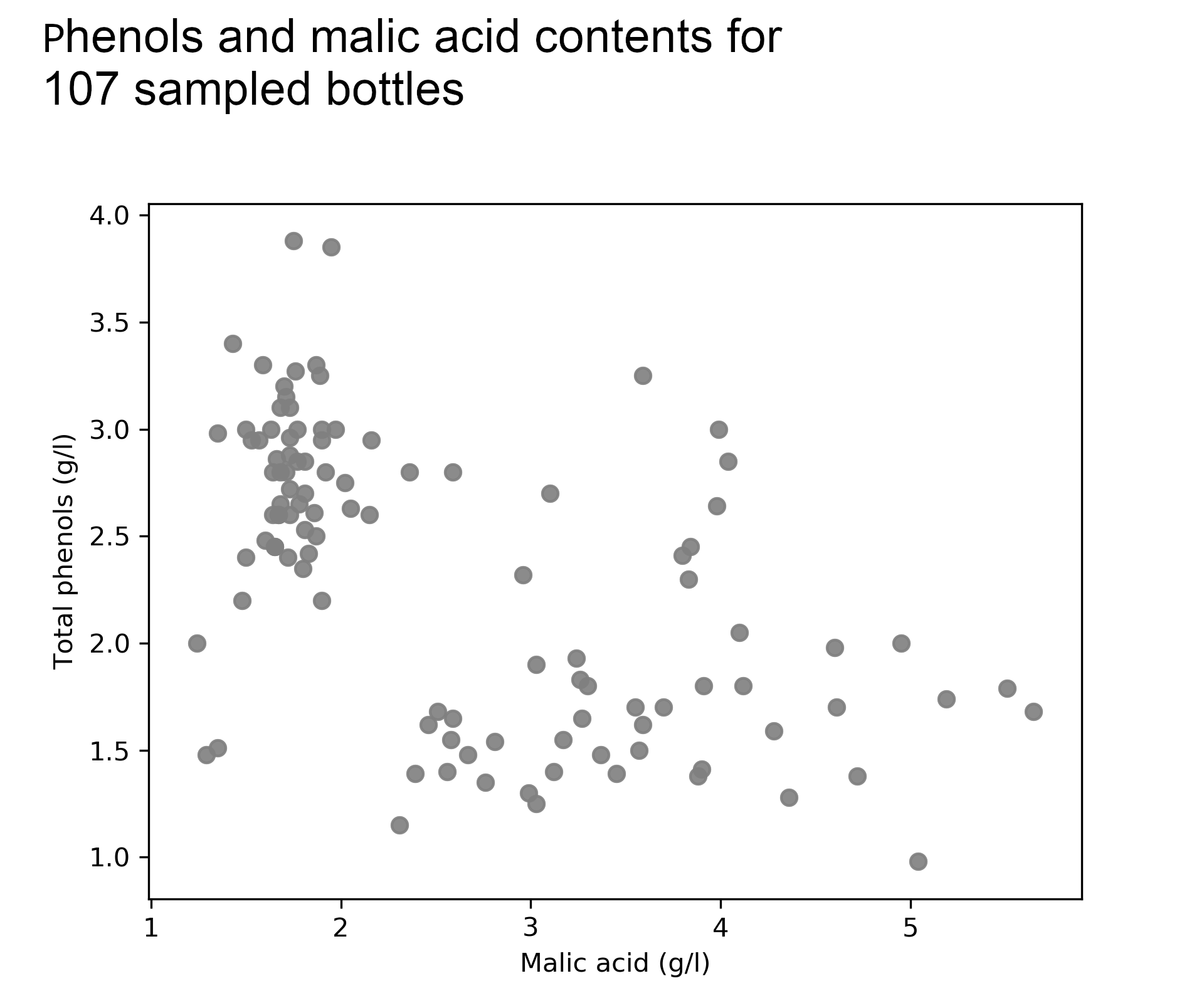
I pair up a popular wine data set with another imaginary story to flesh out the equations above and try to demonstrate why EM is a simple and smart way to solve a difficult problem. The data set is available on the UCI data set repo.
Kate’s restaurant menu features a popular bottle of red wine that she has purchased from the same local Italian winemaker for years. Lately, she has noticed a lack of consistency in taste and quality across bottles and she suspects that the winemaker may use different types of grapes — also called cultivars — perhaps in an attempt to cut costs.
She runs sample analyses for random bottles and investigates two attributes that drive taste, phenols and malic acid. Although the supplier denies any change in the underlying grapes, she suspects that new bottles have lower phenolic concentration and more malic acid than the traditional bottles.
To test her hypothesis Kate uses a Gaussian mixture model with 2 components to model phenols and malic acid. If the resulting components seem totally random she will reject her hypothesis but if not, she will urge her supplier to be more transparent about product sourcing and she will have a tool to identify the cultivars for new bottles.
Details of E and M
The E step computes the posterior distribution using Bayes’ formula detailed in equation 3.2. It assigns an observation to a component by dividing the component joint probability by all components’ probabilities. The higher a component’s joint probability, the higher its membership assignment.
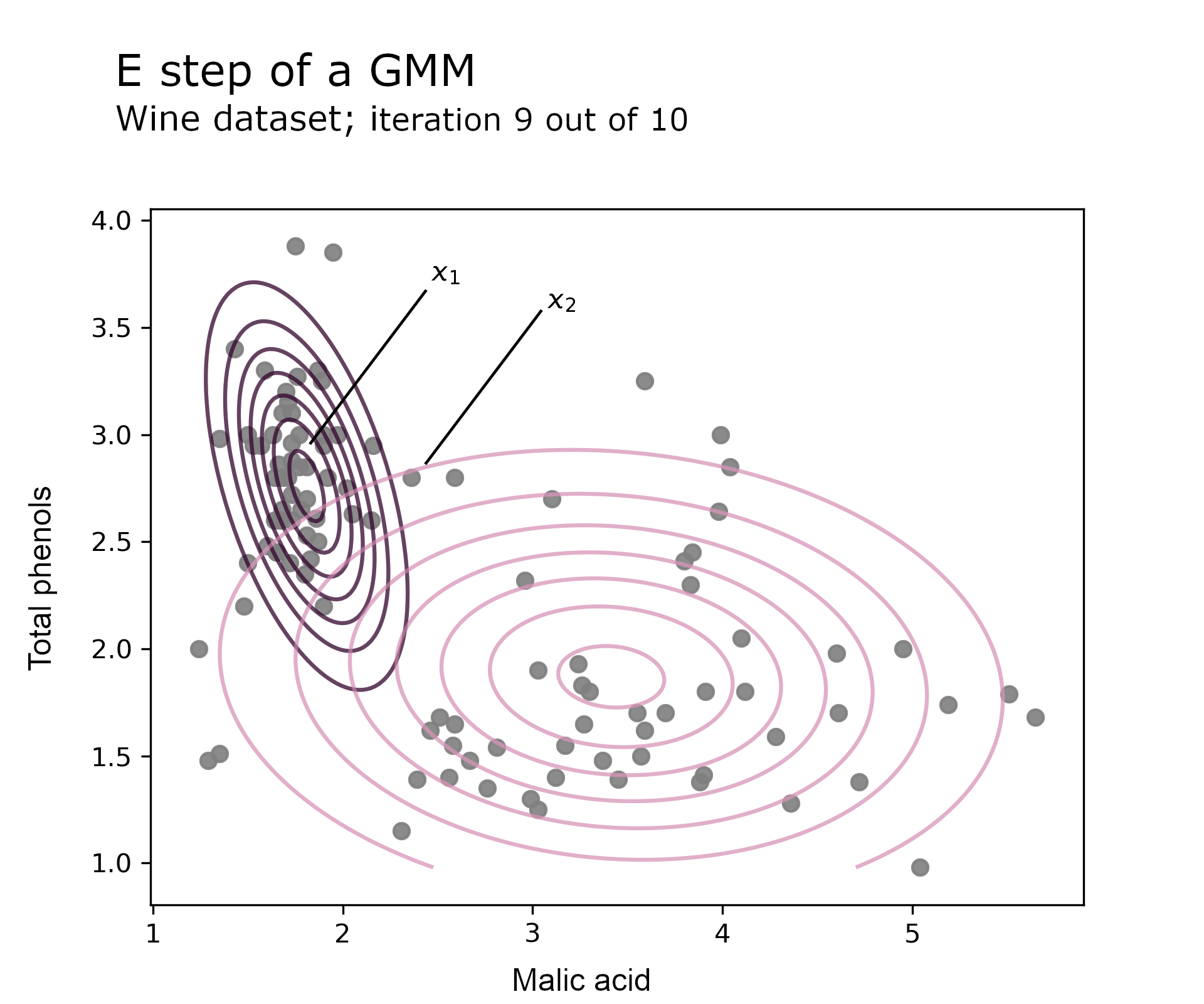
In this example it turns out that prior probabilities are roughly equal as $\pi_1 = 0.49$ so the likelihood drives most of the membership assignment. On the E step chart below, the contour plots represent the Gaussian likelihood for each component. The code uses a single run of EM (no restarts) and converges after 10 iterations. The chart focusses on the 9th round.
Observation $x_1$ lies close to $\mu_1$ i.e. has a high component likelihood, which means that the component 1 posterior probability is close to 1. On the contrary, observation $x_2$ is several standard deviations away from the mean of both components, so membership assignment will sit on the fence i.e. the posterior probability is around to 0.5.
The code implementation was described in part 1 of these blog posts. The Gaussian likelihood function below is plugged into the main e_step function.
def gaussian_likelihood(c: int, mixture_params: Tuple[Any], X: np.array) -> np.array:
    """
    Multivariate normal function using the mixture parameters.
    Implements equation 3.2.

    Args:
      c: Component index
      mixture_params: Distribution parameters i.e. prior proba, mean and variance
      X: Observations (N, D).

    Returns:
         Gaussian probability density for X
    """
    mu = mixture_params[1]
    sigma = mixture_params[2]
    return mvn(mu[c], sigma[c]).pdf(X)

e_step_gaussian = e_step(likelihood=gaussian_likelihood)
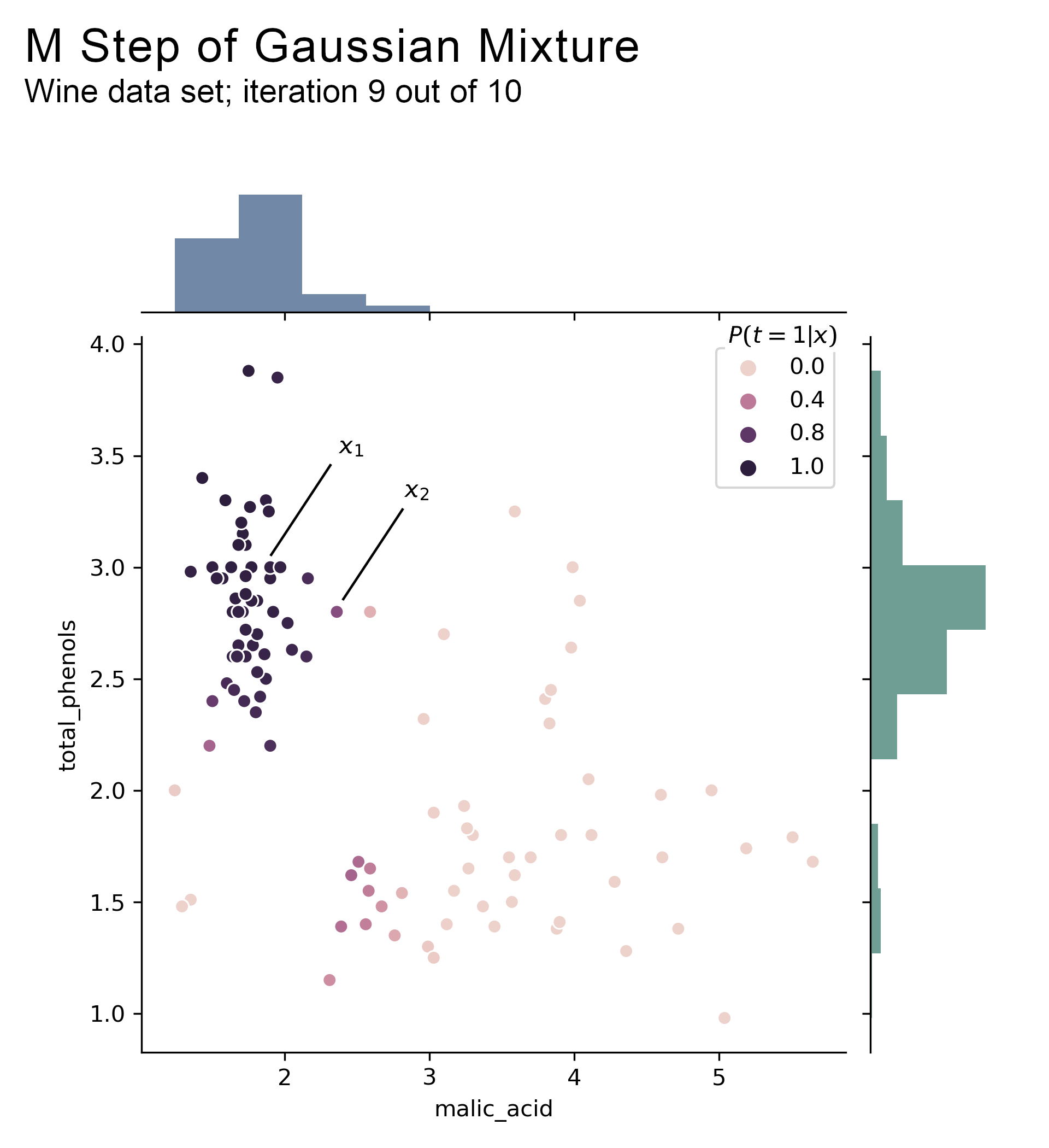
The next chart shows the posterior probabilities computed above, which become the input for the M step. The probabilities are for component 1 i.e. a proba close to 1 means that the observation is assigned to component 1.
The side histograms represent value counts weighted by the posterior probabilities, which is a visual representation of the solution to $\mu_1$ in equation 3.4. The mean for malic acid at the top is around 2 and the mean for phenols on the right side is around 3, suggesting that $\mu_1$ is close to (2.0, 3.0) on iteration 9. Indeed, the computed value is (1.8, 2.8).
The code is broadly similar as before, with mixture_m_step_gaussian replacing mixture_m_step_poisson.
def mixture_m_step_gaussian(X: np.array, q: np.array, C: int, D: int) -> Tuple[Any]:
    """
      M step solution for GMM parameters \mu and \sigma
      i.e. equations 3.4 and 3.6

      Args:
        X: data (N, D).
        q: posterior probabilities (N, C).

      Returns:
        the updated parameters.
    """
    # Equation 3.4
    mu = q.T.dot(X) / np.sum(q.T, axis=1, keepdims=True)

    sigma = np.zeros((C, D, D))
    # Equation 3.6
    for c in range(C):
        delta = (X - mu[c])
        sigma[c] = (q[:, [c]] * delta).T.dot(delta) / np.sum(q[:, c])
    return (mu, sigma)

m_step_gaussian = m_step(mixture_m_step_gaussian)
The power of the posterior
Looking at the model fit with different numbers of components confirms Kate’s initial hypothesis. A single Gaussian does not fit the data distribution well as there are barely any observations around its mean. With 3 components, the 3rd Gaussian unnecessarily overlaps the other two. If $K=2$, the first component with high phenols and lower malic acid would correspond to the better wine that the supplier has historically shipped to Kate.
Model selection metrics support the assumption that there is more than one component as AIC and BIC drop sharply between 1 and 2 components. The reduction in AIC/BIC after 2 components, albeit slower than after 1 component, means that there may be more than 2 grape types, which does not exactly corroborate the previous “eyeballing” interpretation.

With confidence in her Gaussian mixture model, Kate now needs to identify if a new shipment corresponds to bottles of type 1 or 2. The posterior probabilities provide a great way to “operationalise” a GMM. After measuring malic acid and phenol contents for a batch of bottles $X_{new}$, she can just feed the data into $P(t=1 \vert X_{new})$. If probabilities are low then the bottles likely come from component 2 and she will take the necessary actions.
The posterior probas are more than just a cog in the EM machine. They can be a tool to organise and summarise data observations into one of the K components, which is why discrete models and GMM in particular are widely used for clustering.
For example, scikit-learn’s GMM implementation has a few prediction methods that refer to classification using the fit model’s posterior probabilities. More generally, the posterior probas encode data from a complex space with potentially many dimensions into a simpler space, which the next latent model example will illustrate.
Beyond discrete mixture models
Changing some assumptions
EM can be extended to address other, potentially more difficult modelling problems, which this section provides a non-exhaustive overview of.
The discrete mixture case can be easily extended to other probability distributions of the exponential family and to continuous latent probability spaces. An example of continuous latent space is probabilistic PCA (PPCA), an alternative to traditional Principal Component Analysis that is robust to missing observations.
An assumption that often must be dropped in applied work is that observations are independently drawn from the same process. Hidden Markov Models (HMM) deal with correlated $x$’s and can be optimised with what is essentially a special case of EM.
Next, one can assume that, unlike in equation 3.2, the posterior probability distribution $P(t \vert x)$ is too complex to have a closed-form solution. EM still applies if we approximate it with a simpler distribution with a closed form, which allows for complex cases, for example topic modelling with Latent Dirichlet Allocation (LDA).
This so-called variational EM approach is also used to estimate Maximum A Posteriori (MAP) parameters for latent models like GMM. The usual benefits of Bayesian inference then apply to latent variable models by providing a probability distribution for the parameters, and thus for the predictions.
Kate may find the above GMM limited in cases when posterior probas are close to 0.5. Knowing that a bottle’s membership assignment to cluster 1 is 0.6 only tells her that the most likely cluster is 1. How certain can she be that this value is not, say 0.52 or 0.45? Bayesian GMM can provide an answer to that question and better inform her decision process.
So far, probability distributions can be applied directly to the observed value. Relaxing this assumption provides the ability to apply a transformation function between the data space and the latent space, which is useful for problems where data dimensions have non-linear correlations, e.g. image pixels or sound waves. The next part describes a solution to optimise such models which bears a resemblance to EM.
Variational Autoencoders
VAEs are a recent type of machine learning models that have expanded the applications of generative models to new data types, including images and audio signals, by combining variational Bayes with deep learning architectures. Expectation-Maximization and VAE both maximise a lower bound of the maximum likelihood function so many previously uncovered aspects will come in handy.
The following highlights some of the key similarities between EM and VAEs. However, it is not a comprehensive treatment of VAEs, which can be found in the original VAE article - see references.
Continuous latent space
The diagram below compares the generative process from the latent space to the data space for VAEs vs discrete mixture models.

With a discrete latent space the number of parameters to estimate depends on the number of mixture components. With a continuous space there is no finite number of mixture components so instead, the parameters to estimate are the coefficients of the transformation from $t$ to the parameters of the mixture random variable, e.g. probability of success $p$ for a Bernoulli RV.
The number of parameters thus depends on the transformation function, $f$. It can be as simple as a logit although most applications would use deep neural networks for non-linear data structures like images or sound waves. The mixture distribution is said to be parametrised by the function $f$, which in the absence of a closed-form solution, is typically optimised with stochastic gradient descent (SGD).
For a given latent variable $t$ and a set of weights $\theta$ the MNIST digit generated is assumed to be distributed as
\[x_i \sim \rm Bernoulli(f(t \vert \theta))\]and as with previous examples the log-likelihood can be marginalised out
\[\begin{equation} \begin{aligned} \sum_{i=1}^N \log P(x_i|\theta) & = \sum_{i=1}^N \log \int P(x_i, t \vert \theta) dt \\ & = \sum_{i=1}^N \log \int P_{\mathcal{N}}(t \vert 0, I) * P_{\rm Bernoulli}(x_i \vert f(t \vert \theta)) dt \end{aligned} \end{equation} \tag{4.1}\]Maximum Likelihood Estimation
The parameters of the transformation function will be approximated rather solved analytically because this function has no closed-form solution.
Removing the constraints associated with analytical solutions gives hope for direct optimisation of the log-likelihood rather than EM. The integral inside the objective function, which would cause so much pain when solved by hand, can be approximated with a sampling method to then apply SGD. For example, using Monte Carlo approximation, equation 4.1 becomes
\[\sum_{i=1}^N \log P(x_i|\theta) \approx \sum_{i=1}^N \log \sum_{m=1}^M P_{\rm Bernoulli}(x_i \vert f(t_m \vert \theta)) dt\]where $t_m$ refers to the $m$’th sample from a normalised Gaussian. The expression to evaluate is an unbiased estimator of the integral of the log-likelihood, which is good but not necessarily efficient.
Using a sentence from the original paper in a different context, “this series of operations can be expressed as a symbolic graph in software like Tensorflow or Chainer, and effortlessly differentiated wrt the parameters $\theta$”, and I would add “although painfully computed unless using quantum machines from the future.”
The additional bit refers to sampling from $t$ being inefficient because it requires a very large number of samples to make marginal improvements. Most samples from $t$ will contribute next to nothing to the observations $x$, which means that gradients will take a lot of time to converge. As a reminder, stochastic gradient descent nudges gradients in the right direction by getting feedback from the loss function. Here feedback will often be poor as the loss function does not get many examples of correct $t$ values.
It is like a tourist asking for directions by enumerating all the wrong routes to locals. There is a large number of routes to rule out before one finds the correct itinerary. If the symbolic graph, i.e. the tourist, could make more educated suggestions, then it could get to its destination faster. The lower bound addresses this issue via the posterior function.
Lower bound
EM and the VAE are connected via the lower bound as they both aim to maximise a lower bound on the log-likelihood of the joint probability. The derivation for equation 2.1 in the previous part of this article also applies to continuous latent models with minimum changes. $q$ still refers to any probability distribution over the hidden variables
\[\sum_{i=1}^N \log P(x_i|\theta) = L(\theta) + KL(q(t)\parallel p(t|x,\theta))\]As with discrete mixtures, the objective function can be written as the sum of a lower bound and a measure of the divergence between the latent variable posterior distribution and the arbitrary distribution $q$. In the handwritten digit example, the posterior probability returns the most likely latent value $t$ for a given MNIST picture.
The lower bound is
\[L(\theta) = \sum_i^N\{ \int q(t) \log P(x_i, t) dt - \int q(t) \log q(t) dt \} \tag{4.2}\]We will assume to have a good approximation of the posterior distribution, $q_{magic}(t \vert x_i) \approx p(t_i \vert x_i)$. $q_{magic}$ is a temporary placeholder to focus on the similarities with EM. Solving for $\theta$ then corresponds to
\[\DeclareMathOperator*{\argmax}{argmax} \argmax\limits_{\theta} L(\theta) = \sum_i^N\ \int q_{magic}(t) \log P(x_i, t) dt\]As with the discrete mixture case, the above is close to the observed component likelihood function with $q_{magic}$ filling in the gap for the latent variable. Applying the distributional assumptions for the MNIST example and approximating the integral gives
\[\approx \sum_i^N\ \sum_{m=1}^M q_{magic}(t_m) \log \{ P_{\mathcal{N}}(t \vert 0, I) * P_{\rm Bernoulli}(x_i \vert f(x_i \vert t, \theta)) \} dt \tag{4.3}\]This quantity, which can be evaluated with stochastic gradient methods, contrasts with the direct log-likelihood function above because sampling over the approximate posterior is more efficient than sampling over the prior distribution. Instead of looping through many unlikely $t$ values, the model is forced to loop through the most likely latent values that generated the observations, which $q_{magic}$ does as an approximation of the posterior.
Finally, the VAE optimises a rearranged version of the lower bound that is more aligned with the machine learning view. Moving the prior probability $p(t)$ to the RHS expression then equation 4.2 can be written
\[\sum_i^N\ \int q(t \vert x_i) \log P_{\rm Bernoulli}(x_i \vert f(x_i \vert t, \theta)) dt - KL(q(t \vert x_i) \parallel P_{\mathcal{N}}(t \vert 0, I)) \tag{4.4}\]The previous form in 4.2, sometimes called “free energy”, can be seen as maximising the observed component function even as latent components are not observed. As described with the Poisson mixture, the posterior $q$ is the best substitute for the unobserved latent variable.
The new form, sometimes called “penalised model fit”, can be seen as a regularised function, e.g. as with the Lasso regression where L1 acts as the regularisation term. The LHS expression measures the model fit through the marginal probability, while the KL divergence is a regularisation term as it forces the posterior approximation close to an isometric (0-mean and identity covariance matrix) Gaussian.
Variational Bayes
EM sets $q$ equal to the posterior $p(t \vert x)$ so the lower bound is equal to the log-likelihood using Bayes’ formula, which was possible in the presence of a closed-form solution for mixture distributions. With the complex function $f$ it would be hard because the denominator of Bayes’ formula is an integral of a function with no closed-form solution.
The VAE optimisation scheme proposed in the article, called Auto Encoding Variational Bayes (AEVB), differs from EM because it uses an approximation of the posterior instead of plugging the result from E into the M objective function. At a high level, AEVB sets q to be a simple random variable, typically a symmetric Gaussian distribution, parametrised by a neural network -based transformation $g$ with weights $\phi$. The lower bound $L(\theta, \phi)$ is then a function of two sets of parameters optimised jointly with batch gradient descent methods.
The reason why this scheme converges to a local optimum is beyond the scope of this text and can be found in the stochastic variational inference literature. The implementation details are well covered in the original VAE paper and most neural network packages documentation. The following glosses over some key implementation aspects using a detailed formulation of the objective function $L$, which I find is often missing.
Finally, it took me some time to comprehend how AEVB approximates the unseen posterior with a parameterised function. What I found unsettling - probably because I did not come to VAEs with a background in variational inference - is that the variational function is an input into another function, $f$, whose parameters are also estimated. However, when you think about it, this type of inference problems is similar to other statistical estimation — guess the values of invisible parameters by doing stuff on the visible output.
The variational assumptions are
\[q(t \vert \ x_i) \sim \mathcal{N} (\mu, \Sigma)\] \[\mu = g_{\mu} (x_i \vert \phi)\] \[\Sigma = g_{\Sigma} (x_i \vert \phi)\]The first line means that $q$, which approximates the complicated posterior, is set to be a Gaussian distribution. Its covariance $\Sigma$ is symmetric i.e. latent variables are assumed independent. It is unlikely to be true but it reduces the number of parameters vs a free covariance matrix. The second and third lines mean that $g$ has two outputs corresponding to the two parameters of the distribution that it parameterises, $q$.
Plugging this into the lower bound,
\[L(\theta, \phi) = \sum_i^N\ \int P_{\mathcal{N}}(t \vert \mu, \Sigma) \log P_{\rm Bernoulli}(x_i \vert f(x_i \vert t, \theta)) dt - KL(P_{\mathcal{N}}(t \vert \mu, \Sigma) \parallel P_{\mathcal{N}}(t \vert 0, I)) \tag{4.5}\]The integral is approximated as before but M=1. Using only one sample may result in a high variance estimator however more samples would be computationally costly as they must be passed into the transformation function $f$ to estimate their lower bound values. So there’s a trade-off, which the authors seem to have solved empirically — quote is from the 2014 paper.
In our experiments we found that the number of samples per datapoint can be set to 1 as long as the minibatch size was large enough, e.g. size equal to 100.
If $t^{\ast}$ refers to that one sample drawn from ${\mathcal{N}}(\mu, \Sigma)$, equation 4.5 can be approximated as
\[\approx \sum_i^N\ \log P_{\rm Bernoulli}(x_i \vert f(x_i \vert t^{\ast}, \theta)) dt - KL(P_{\mathcal{N}}(t \vert \mu, \Sigma) \parallel P_{\mathcal{N}}(t \vert 0, I))\]To be accurate the sample $\epsilon$ is drawn from ${\mathcal{N}}(0, I)$ then multiplied by $\Sigma$ and added to $\mu$. This location-scale transformation does not change $t$’s distribution but allows $\phi$ to remain fixed during backpropagation. Without this so-called “reparameterization trick”, we are trying to compute the gradient of a parameter that has randomness, which is not possible. This transformation can be reflected in the lower bound as
\[\approx \sum_i^N\ \log P_{\rm Bernoulli}(x_i \vert f(x_i \vert t = g_{\mu} (x_i \vert \phi) + g_{\Sigma} (x_i \vert \phi) * \epsilon^{\ast}, \theta)) dt - KL(P_{\mathcal{N}}(t \vert \mu, \Sigma) \parallel P_{\mathcal{N}}(t \vert 0, I)) \tag{4.6}\]The encoder-decoder framework helps make sense of the LHS nested conditional probability. Starting with the innermost condition, $g_{\mu} (x_i \vert \phi) + g_{\Sigma} (x_i \vert \phi) * \epsilon^{\ast}$ is the encoder i.e. mapping $x_i$ to the latent space. Then $f(x_i \vert t)$ is the decoder i.e. the transformation from $t$ to the observed space, and $P_{\rm Bernoulli}$ is the distributional assumption for the marginal likelihood.
Lower bound code example
The Keras blog provides a slick code implementation of the above objective function 4.6.
def vae_loss(x, x_decoded_mean):
    xent_loss = objectives.binary_crossentropy(x, x_decoded_mean)
    kl_loss = - 0.5 * K.mean(1 + z_log_sigma - K.square(z_mean) - K.exp(z_log_sigma), axis=-1)
    return xent_loss + kl_loss

vae.compile(optimizer='rmsprop', loss=vae_loss)
In vae_loss, x_ent corresponds to the reconstruction loss and kl_loss is the regularisation term. The former uses binary cross-entropy, which is the information theoretical equivalent of a Bernoulli density, best seen by looking at the Keras source implementation
  # Compute cross entropy from probabilities.
  bce = target * math_ops.log(output + epsilon())
  bce += (1 - target) * math_ops.log(1 - output + epsilon())
  return -bce
The optimiser minimises the loss function, and minimising the inverse of bce is equivalent to maximising the Bernoulli probability density.
In the snippet above, the ground truth $x_i$ is denoted target and the predicted output is denoted x_decoded_mean - “mean” refers to $f(x_i \vert t)$ being both the parameter and the mean of the Bernoulli RV. Then equation 4.6 can be written as follows to emphasize the equivalence with the Keras BCE function
Last, kl_loss implements the closed form solution for the KL divergence of two Gaussians.
Conclusion
Expectation-Maximization finds the parameters of a latent variable model by optimising a substitute for the log-likelihood. It can be applied to many models that are useful to address business problems and is worth knowing for this reason alone. Moreover, popular alternatives minimise the same loss function and share similar principles as EM, e.g. the AEVB.
With EM or related methods, the posterior probability distribution $q(t \vert x)$ is more than a means to an end as its encoding properties can power applications or generate insights. This is probably even more true for recent generative models like VAEs that often support unsupervised learning tasks by training an encoder to organise/cluster unlabelled data.
In the last couple of years, major improvements in the way VAEs build informative latent spaces got us closer to models that can teach us something about the world around us using data.
For example, the BetaVAE forces latent dimensions to represent independent data features simply by cranking up the importance of $LB$’s regularization term. This results in more meaningful latent variables tied to human concepts, e.g. the dimensions of $t$ would represent the height/width/location of the MNIST digit.
While the focus in the ML industry now seems to be around “productionising” models, i.e. monetising the statistical mimicries developed in the last decade to automate high volume/small unit value tasks, I find these new developments exciting and refreshing.
References
Core
- C. Bishop. Pattern Recognition and Machine Learning (PRML).
- Diederik P Kingma and Max Welling (2014). Auto-encoding variational Bayes. https://arxiv.org/abs/1312.6114
- Diederik P Kingma and Max Welling (2019). An introduction to Variational Autoencoders. https://arxiv.org/abs/1906.02691
- Code is hosted on Github, and is mostly based on Martin Krasser’s notebook.
Additional sources
- David Blei, Alp Kucukelbir and Jon D. McAuliffe. Variational Inference: A Review for Statisticians. https://arxiv.org/abs/1601.00670
- For an intuitive guide to VAEs: Brian Keng’s blog article “Variational Autoencoders”. http://bjlkeng.github.io/posts/variational-autoencoders/
- For further details on the probabilistic vs ML perspectives: Jan Altosaar’s blog article “Tutorial - What is a variational autoencoder?”. https://jaan.io/what-is-variational-autoencoder-vae-tutorial/